Predicting subcellular compartments with C-COMPASS

grassp can drive C-COMPASS (Haas et al., Nature Methods 2025), a neural-network classifier that assigns each protein a class contribution over subcellular compartments from fractionation profiles. Because the contributions for a protein sum to 1, C-COMPASS naturally reports multi-localizing proteins.

In this tutorial we run C-COMPASS on the Haas 2025 humanized-liver dataset through grassp, using both the quick median workflow and the paper-faithful per-replicate workflow, and visualize the predictions on a UMAP.

Installation

The C-COMPASS integration is an optional extra (it pulls in TensorFlow/Keras). Install it with:

pip install grassp[ccompass]

TensorFlow currently provides wheels for Python ≤ 3.13, so use a 3.12/3.13 environment. The rest of grassp does not require this extra.

# Spatial and single-cell analysis
import grassp as gr
import scanpy as sc

# Numerical computing
import numpy as np
import pandas as pd
import matplotlib.pyplot as plt

Loading the data

We use gr.ds.load_dataset to pull curated datasets from the grassp portal by name. enrichment="enriched" returns the processed object — for this dataset that is the replicate-median fractionation profile with a precomputed UMAP. The authors’ input marker set is in obs["author_markers"], and their published C-COMPASS assignment is in obs["author_annotation"].

adata = gr.ds.load_dataset("Haas_2025_HumanizedLiver_Chow", enrichment="enriched")
adata

AnnData object with n_obs × n_vars = 6117 × 14
    obs: 'author_gene_symbol', 'ProteinGroups', 'uniprot_id', 'author_markers', 'author_annotation', 'marker_lilley', 'marker_christopher', 'marker_geladaki', 'marker_itzhak', 'marker_villaneuva', 'marker_hein2025', 'marker_hein2025_gt', 'n_replicates_with_minimum_3_fractions', 'n_samples_by_intensity', 'mean_intensity', 'log1p_mean_intensity', 'pct_dropout_by_intensity', 'total_intensity', 'log1p_total_intensity'
    var: 'replicate', 'fraction_order', 'fraction', 'n_proteins_by_intensity', 'log1p_n_proteins_by_intensity', 'total_intensity', 'log1p_total_intensity', 'pct_dropout_by_intensity', 'subcellular_enrichment', 'n_merged_samples', 'enriched_vs'
    uns: 'author_annotation_colors', 'author_markers_colors', 'marker_christopher_colors', 'marker_geladaki_colors', 'marker_hein2025_colors', 'marker_hein2025_gt_colors', 'marker_itzhak_colors', 'marker_lilley_colors', 'marker_villaneuva_colors', 'neighbors', 'pca', 'umap'
    obsm: 'X_pca', 'X_umap', 'X_umap3D'
    varm: 'PCs'
    layers: 'original_intensities', 'pvals'
    obsp: 'connectivities', 'distances'

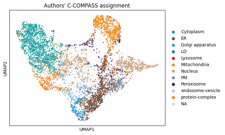
The authors’ published C-COMPASS assignment separates cleanly on the UMAP:

sc.pl.umap(adata, color="author_annotation", title="Authors' C-COMPASS assignment")

Inspecting the C-COMPASS parameters

gr.tl.ccompass_default_params() returns the hyperparameters C-COMPASS will use (network, training, and the reliability filter). Every field is overridable via the nn_params argument (a dict, a NeuralNetworkParametersModel, or a path to a YAML file). grassp defaults NN_optimization="short" to match the paper.

gr.tl.ccompass_default_params()

NeuralNetworkParametersModel(upsampling=True, upsampling_method='noisedaverage', upsampling_noise=2, svm_filter=False, mixed_part=4, mixed_batch=0.05, NN_optimization='short', NN_activation='relu', class_activation='linear', class_loss='mean_squared_error', optimizers=['adam', 'rmsprop', 'sgd'], NN_epochs=20, rounds=3, subrounds=10, reliability=95)

Simple workflow (median profiles)

The enriched object has a single (median) profile per protein, so we call gr.tl.ccompass with aggregate=False: C-COMPASS trains on the marker proteins in author_markers and predicts a compartment for every protein.

Here we deliberately shrink rounds/subrounds so the tutorial runs quickly; the defaults shown above (rounds=3, subrounds=10) reproduce the paper.

fast = {"rounds": 1, "subrounds": 5}
gr.tl.ccompass(adata, marker_key="author_markers", aggregate=False, nn_params=fast)
adata

AnnData object with n_obs × n_vars = 6117 × 14
    obs: 'author_gene_symbol', 'ProteinGroups', 'uniprot_id', 'author_markers', 'author_annotation', 'marker_lilley', 'marker_christopher', 'marker_geladaki', 'marker_itzhak', 'marker_villaneuva', 'marker_hein2025', 'marker_hein2025_gt', 'n_replicates_with_minimum_3_fractions', 'n_samples_by_intensity', 'mean_intensity', 'log1p_mean_intensity', 'pct_dropout_by_intensity', 'total_intensity', 'log1p_total_intensity', 'ccompass'
    var: 'replicate', 'fraction_order', 'fraction', 'n_proteins_by_intensity', 'log1p_n_proteins_by_intensity', 'total_intensity', 'log1p_total_intensity', 'pct_dropout_by_intensity', 'subcellular_enrichment', 'n_merged_samples', 'enriched_vs'
    uns: 'author_annotation_colors', 'author_markers_colors', 'marker_christopher_colors', 'marker_geladaki_colors', 'marker_hein2025_colors', 'marker_hein2025_gt_colors', 'marker_itzhak_colors', 'marker_lilley_colors', 'marker_villaneuva_colors', 'neighbors', 'pca', 'umap', 'ccompass_nn_params', 'ccompass_categories', 'ccompass_colors'
    obsm: 'X_pca', 'X_umap', 'X_umap3D', 'ccompass_contributions'
    varm: 'PCs'
    layers: 'original_intensities', 'pvals'
    obsp: 'connectivities', 'distances'

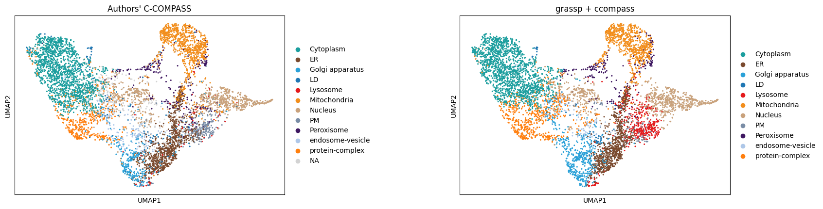
ccompass writes the winning compartment to obs["ccompass"], the full class-contribution matrix to obsm["ccompass_contributions"], and the compartment order to uns["ccompass_categories"]. The predicted map closely matches the authors’ assignment:

sc.pl.umap(
    adata,
    color=["author_annotation", "ccompass"],
    title=["Authors' C-COMPASS", "grassp + ccompass"],
    wspace=0.5,
)

Because the output is a probability-like vector, we can also weight each point by its prediction confidence (the top class contribution) using grassp’s umap_prob:

adata.obs["ccompass_conf"] = adata.obsm["ccompass_contributions"].max(axis=1)
gr.pl.umap_prob(adata, color="ccompass", color_prob="ccompass_conf")

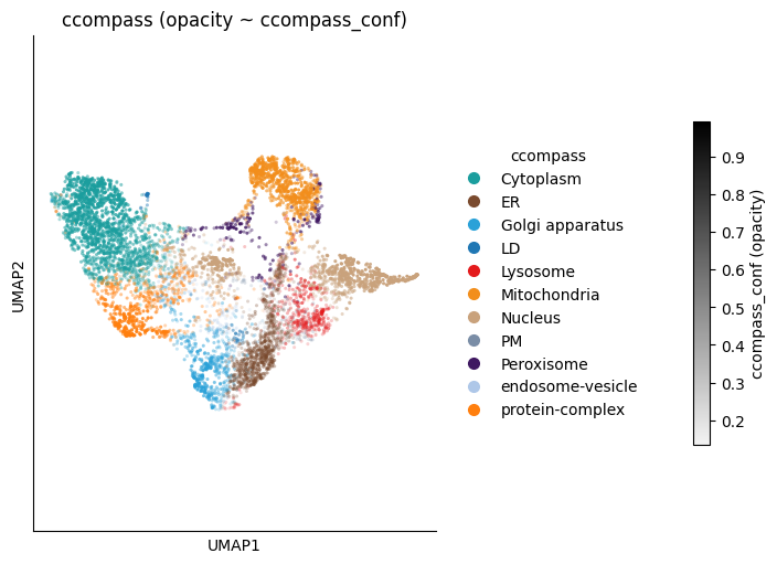
<Axes: title={'center': 'ccompass (opacity ~ ccompass_conf)'}, xlabel='UMAP1', ylabel='UMAP2'>

Faithful workflow (per-replicate + reliability filtering)

The paper trains a network per replicate and then applies a reliability filter (fCC) that removes spurious contributions using cross-replicate behaviour. This needs the individual replicates, which we get with enrichment="raw".

raw = gr.ds.load_dataset("Haas_2025_HumanizedLiver_Chow", enrichment="raw")
raw

AnnData object with n_obs × n_vars = 8833 × 42
    obs: 'author_gene_symbol', 'ProteinGroups', 'uniprot_id', 'author_markers', 'author_annotation', 'marker_lilley', 'marker_christopher', 'marker_geladaki', 'marker_itzhak', 'marker_villaneuva', 'marker_hein2025', 'marker_hein2025_gt'
    var: 'replicate', 'fraction', 'fraction_order'
    uns: 'author_annotation_colors', 'author_markers_colors', 'condition', 'marker_christopher_colors', 'marker_geladaki_colors', 'marker_hein2025_colors', 'marker_hein2025_gt_colors', 'marker_itzhak_colors', 'marker_lilley_colors', 'marker_villaneuva_colors', 'replicates'

C-COMPASS’s classification input is normalized so each replicate profile sums to 1 (missing values treated as 0), and proteins seen in fewer than two replicates are dropped. We apply that normalization, then run ccompass with replicate_key="replicate" and aggregate=True (and scale=False, since we normalized ourselves).

def area_normalize_per_replicate(a):
    """missing -> 0, then normalize each replicate profile to sum 1; keep proteins in >=2 reps."""
    X = np.asarray(a.X, dtype=float)
    reps = a.var["replicate"].values
    identified = np.zeros(a.n_obs, dtype=int)
    for g in np.unique(reps):
        cols = np.where(reps == g)[0]
        block = np.nan_to_num(X[:, cols], nan=0.0)
        identified += (block != 0).any(axis=1).astype(int)
        s = block.sum(axis=1, keepdims=True)
        X[:, cols] = np.divide(block, s, out=np.zeros_like(block), where=s > 0)
    a.X = X
    return a[identified >= 2].copy()


raw = area_normalize_per_replicate(raw)
raw

AnnData object with n_obs × n_vars = 7871 × 42
    obs: 'author_gene_symbol', 'ProteinGroups', 'uniprot_id', 'author_markers', 'author_annotation', 'marker_lilley', 'marker_christopher', 'marker_geladaki', 'marker_itzhak', 'marker_villaneuva', 'marker_hein2025', 'marker_hein2025_gt'
    var: 'replicate', 'fraction', 'fraction_order'
    uns: 'author_annotation_colors', 'author_markers_colors', 'condition', 'marker_christopher_colors', 'marker_geladaki_colors', 'marker_hein2025_colors', 'marker_hein2025_gt_colors', 'marker_itzhak_colors', 'marker_lilley_colors', 'marker_villaneuva_colors', 'replicates'

gr.tl.ccompass(
    raw,
    marker_key="author_markers",
    replicate_key="replicate",
    aggregate=True,
    scale=False,
    nn_params=fast,
)
raw

AnnData object with n_obs × n_vars = 7871 × 42
    obs: 'author_gene_symbol', 'ProteinGroups', 'uniprot_id', 'author_markers', 'author_annotation', 'marker_lilley', 'marker_christopher', 'marker_geladaki', 'marker_itzhak', 'marker_villaneuva', 'marker_hein2025', 'marker_hein2025_gt', 'ccompass', 'ccompass_fwinner'
    var: 'replicate', 'fraction', 'fraction_order'
    uns: 'author_annotation_colors', 'author_markers_colors', 'condition', 'marker_christopher_colors', 'marker_geladaki_colors', 'marker_hein2025_colors', 'marker_hein2025_gt_colors', 'marker_itzhak_colors', 'marker_lilley_colors', 'marker_villaneuva_colors', 'replicates', 'ccompass_nn_params', 'ccompass_categories', 'ccompass_colors', 'ccompass_fwinner_colors'
    obsm: 'ccompass_contributions', 'ccompass_fcontributions'

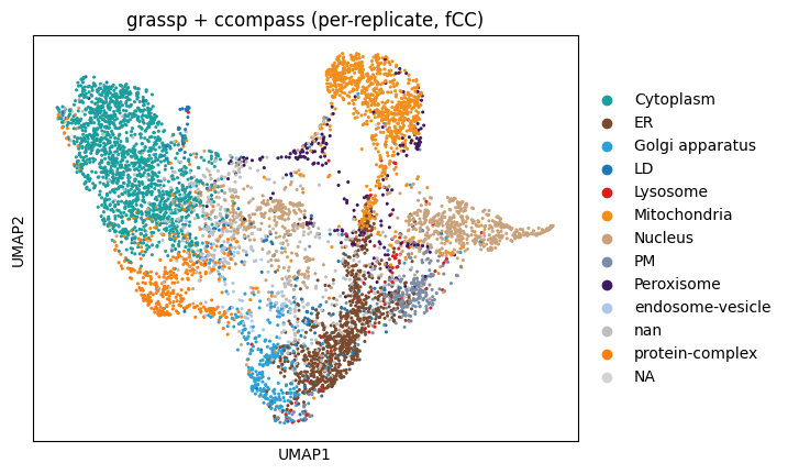
With aggregate=True you additionally get the reliability-filtered contributions in obsm["ccompass_fcontributions"] and the filtered winner in obs["ccompass_fwinner"]. We transfer the filtered winner onto the enriched object (shared UniProt ids) to plot it on the same UMAP:

adata.obs["ccompass_fwinner"] = (
    raw.obs["ccompass_fwinner"].reindex(adata.obs_names).astype("category")
)
gr.pp.set_sensible_compartment_colors(adata, columns=["ccompass_fwinner"])
sc.pl.umap(adata, color="ccompass_fwinner", title="grassp + ccompass (per-replicate, fCC)")

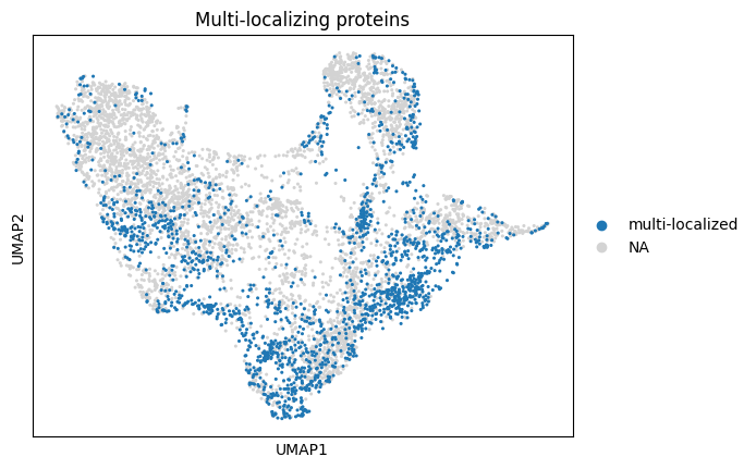
Finally, we flag multi-localizing proteins — those whose second-highest filtered contribution exceeds a threshold — and highlight them on the UMAP:

fcc = np.asarray(raw.obsm["ccompass_fcontributions"], dtype=float)
second = np.sort(fcc, axis=1)[:, ::-1][:, 1]
multi = pd.Series(np.where(second > 0.2, "multi-localized", "single"), index=raw.obs_names)

adata.obs["ccompass_multiloc"] = multi.reindex(adata.obs_names).astype("category")
sc.pl.umap(
    adata,
    color="ccompass_multiloc",
    groups=["multi-localized"],
    title="Multi-localizing proteins",
)

How well does this match the published results?

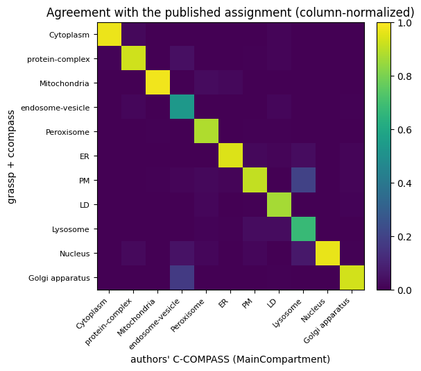
obs["author_annotation"] holds the authors’ published C-COMPASS assignment (their MainCompartment), so we can compare grassp’s per-protein prediction directly to the paper’s output.

The agreement is high but not perfect, for two reasons: (1) shorter training — to keep this tutorial fast we used far fewer rounds/subrounds than the paper (the reduced fast settings above), so there is less ensemble averaging and the prediction is noisier; and (2) the network is stochastic, so even two full runs are never identical. Training with the defaults (rounds=3, subrounds=10, from ccompass_default_params) closes most of the gap and reproduces the authors’ assignments at ~96% (see the C-COMPASS validation in the grassp paper).

# Compare grassp's prediction to the authors' published C-COMPASS assignment.
ref = adata.obs["author_annotation"]
pred = adata.obs["ccompass_fwinner"]
mask = ref.notna() & pred.notna()
acc = (pred[mask].astype(str) == ref[mask].astype(str)).mean()
print(f"agreement with the authors' C-COMPASS assignment: {acc:.1%}  (n={int(mask.sum())})")

cats = list(adata.uns["ccompass_categories"])
ct = (
    pd.crosstab(pred[mask].astype(str), ref[mask].astype(str), normalize="columns")
    .reindex(index=cats, columns=cats)
    .fillna(0.0)
)
fig, ax = plt.subplots(figsize=(6, 5))
im = ax.imshow(ct.values, cmap="viridis", vmin=0, vmax=1)
ax.set_xticks(range(len(cats)))
ax.set_xticklabels(cats, rotation=45, ha="right", fontsize=8)
ax.set_yticks(range(len(cats)))
ax.set_yticklabels(cats, fontsize=8)
ax.set_xlabel("authors' C-COMPASS (MainCompartment)")
ax.set_ylabel("grassp + ccompass")
ax.set_title("Agreement with the published assignment (column-normalized)")
fig.colorbar(im, fraction=0.046, pad=0.04)
plt.show()

agreement with the authors' C-COMPASS assignment: 93.7%  (n=5628)

Median vs. faithful — which to use?

• Median (aggregate=False) is a fast approximation: one network on the collapsed profile, raw contributions only. Good for a quick look.

• Per-replicate (replicate_key=..., aggregate=True) matches the paper: a network per replicate plus the reliability (fCC) filter, which uses replicate reproducibility to separate genuine localization from noise — giving cleaner assignments and multi-localization calls.

Use the median workflow to explore, and the per-replicate workflow when you want results that reproduce the published C-COMPASS output.

Run C-COMPASS on 100+ other datasets

This exact workflow runs on any dataset in the grassp data portal, which hosts over 100 curated spatial-proteomics datasets. Browse them at grassp.apps.czbiohub.org/datasets and just swap the name passed to gr.ds.load_dataset — nothing else changes:

adata = gr.ds.load_dataset("<dataset_name>")                     # processed profiles (+ UMAP)
raw   = gr.ds.load_dataset("<dataset_name>", enrichment="raw")   # per-replicate profiles

From there, the same gr.tl.ccompass calls, plots, and comparisons apply.