pRoloc integration: for grassp users

pRoloc is an R/Bioconductor framework for spatial proteomics. It and grassp have overlapping functionality and hold nearly the same data model, but they share no file format, making it difficult to move data or compare results between the two.

grassp and pRoloc exchange objects as h5ad in both directions, to enable seamless integration. For example, you could preprocess and plot in Python, hand the object to R for pRoloc’s classifiers, and read it back to Python. What comes back is as close to what you sent as the two data models allow, including the results of pRolocs classification. Practically this opens the possibility to use functionality that is not shared between the two frameworks, such as BANDLE in pRoloc for differential localization detection, or the independent diffusion annotation approach in grassp (see the diffusion tutorial).

Note

This tutorial is for someone who works primarily in Python and wants to use a specific pRoloc functionality. If you work primarily in R, read the companion tutorial instead: pRoloc integration: for pRoloc users. It explains how you can load any of the over 100 datasets on the grassp portal into R, and analyze/vizualise with pRoloc.

What this tutorial does

1. Load a dataset and pick a marker set.

2. Write it out as a plain h5ad.

3. Run pRoloc’s SVM and k-NN in R (the R code is shown; its output ships with this tutorial so the notebook builds without R).

4. Read the results back with anndata.read_h5ad and plot them.

5. Merge them onto a session you already have instead.

Installation

grassp comes with functionality to read data directly from R’s native .Rmd format or .h5ad files exported by our R companion package, grasspio, that lives in the same repository. To install the R package:

install.packages(c("remotes", "BiocManager"))
BiocManager::install(c("pRoloc", "rhdf5"))
remotes::install_github("czbiohub-sf/grassp", subdir = "r/grasspio")

grasspio uses the scVerse package anndataR, to convert AnnData files into in-memory R objects under the hood.

import warnings

import anndata
import matplotlib.pyplot as plt
import numpy as np
import scanpy as sc

import grassp as gr

/Users/mfrank/code/grassp/.venv-dev/lib/python3.12/site-packages/tqdm/auto.py:21: TqdmWarning: IProgress not found. Please update jupyter and ipywidgets. See https://ipywidgets.readthedocs.io/en/stable/user_install.html
  from .autonotebook import tqdm as notebook_tqdm

Loading the data

Currie_2024_AC16_Control is a LOPIT-DC experiment on AC16 cardiomyocytes: 2538 proteins across 10 fractions, with each protein’s profile already normalised to sum to 1. Here we load that dataset from the grassp data portal with the load_dataset helper.

adata = gr.ds.load_dataset("Currie_2024_AC16_Control")
adata

AnnData object with n_obs × n_vars = 2538 × 10
    obs: 'protein_name', 'gene_symbol', 'author_annotation', 'author_markers', 'bandle_probability', 'dl_candidate', 'author_markers_data10', 'marker_lilley', 'marker_christopher', 'marker_geladaki', 'marker_itzhak', 'marker_villaneuva', 'marker_hein2025', 'marker_hein2025_gt', 'n_detected', 'n_samples_by_intensity', 'mean_intensity', 'log1p_mean_intensity', 'pct_dropout_by_intensity', 'total_intensity', 'log1p_total_intensity', 'unsupervised_annotation', 'harmonized_annotation_propagated', 'harmonized_annotation_propagated_probability'
    var: 'development_stage', 'tissue', 'sex', 'organism', 'disease', 'cell_line', 'cell_type', 'fraction', 'fraction_order', 'subcellular_enrichment', 'n_proteins_by_intensity', 'log1p_n_proteins_by_intensity', 'pct_dropout_by_intensity', 'n_merged_samples', 'enriched_vs', 'enrichment_strategy', 'mass_spectrometry_method', 'cell_type_ontology_term_id', 'perturbation', 'disease_ontology_term_id', 'organism_ontology_term_id', 'sex_ontology_term_id', 'development_stage_ontology_term_id', 'tissue_ontology_term_id', 'cell_line_ontology_term_id', 'tissue_type', 'tissue_general_ontology_term_id', 'tissue_general', 'organ_ontology_term_id', 'organ', 'system_ontology_term_id', 'system'
    uns: 'author_annotation_colors', 'author_markers_data10_colors', 'dl_candidate_colors', 'harmonized_annotation_propagated_colors', 'marker_christopher_colors', 'marker_geladaki_colors', 'marker_hein2025_colors', 'marker_hein2025_gt_colors', 'marker_itzhak_colors', 'marker_lilley_colors', 'marker_villaneuva_colors', 'neighbors', 'pca', 'publication_authors', 'publication_date', 'publication_doi', 'publication_journal', 'publication_title', 'schema_reference', 'schema_version', 'serves_as_reference', 'title', 'umap', 'unsupervised_annotation_colors'
    obsm: 'X_pca', 'X_umap', 'X_umap3D', 'harmonized_annotation_propagated_one_hot_labels', 'harmonized_annotation_propagated_probabilities'
    varm: 'PCs'
    layers: 'log_intensities', 'original_intensities', 'pvals'
    obsp: 'connectivities', 'distances'

Datasets in the grassp data portal come with several published marker sets. We’ll use Lilley’s, the one pRoloc::pRolocmarkers() provides, and copy it to obs["markers"] — the column name every pRoloc function defaults to.

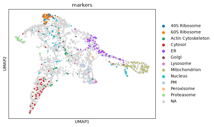
Then we will plot a umap representation of the dataset colored by the marker proteins. One difference of grassp to pRoloc is that dimensionality reduction is separated from plotting and the coordinates are saved with the object. So sc.pl.umap() only does plotting, reusing the stored coordinates in adata.obsm["X_umap"]. Also notice that we are able to use scanpy functions interleaved with grassp functions, because we are using AnnData objects.

adata.obs["markers"] = adata.obs["marker_lilley"]

print(
    f"{adata.obs['markers'].notna().sum()} markers across "
    f"{adata.obs['markers'].nunique()} compartments\n"
)
print(adata.obs["markers"].value_counts().to_string())

sc.pl.umap(adata, color="markers")

403 markers across 12 compartments

markers
Mitochondrion         65
ER                    56
Nucleus               45
60S Ribosome          44
Cytosol               42
PM                    37
Proteasome            31
40S Ribosome          30
Actin Cytoskeleton    28
Lysosome              13
Peroxisome             8
Golgi                  4

Exporting for pRoloc

On the python side exporting just means saving the AnnData object in the .h5ad format. The R package grasspio then reads the file using the anndataR package and translates it into an MSnSet object that pRoloc can use.

This table shows how the attributes of the two in-memory objects correspond:

grassp AnnData	pRoloc MSnSet
.X	exprs() which is the first assayData slot
.obs_names / .var_names	featureNames() / sampleNames()
.obs	fData() scalar columns
.obsm[k], as a DataFrame	fData()[[k]] — a matrix nested inside one column
.var	pData()
.varm[k], as a DataFrame	pData()[[k]] — the same thing on the sample axis
.layers[k]	extra assayData elements
.uns["processing"]	processingData()@processing
everything else in .uns	experimentData()@other$grassp_uns
.obsp / .varp	nothing — eSet has no pairwise slot

Note

The only element that cannot be transferreda are the .obsp / .varp attributes containing the protein-protein graphs, because MSnSet has no pairwise slot that would behave properly when e.g. subsetting the object.

Note

In grassp, unlabelled proteins are labelled NaN by default; in pRoloc they are the literal string "unknown", and pRoloc genuinely needs it (markerMSnSet and unknownMSnSet fail outright on NA). That is one real semantic difference between the frameworks, and it is handled entirely on the R side: grassp_as_msnset(nan_to_unknown = TRUE) fills the sentinel in as the MSnSet is built, and grassp_write_msnset(unknown_to_na = TRUE) strips it on the way back. So the sentinel never touches a file, and you never have to think about it here.

Note

Regarding AnnData layers (AnnData allows to keep multiple version of quantitative matrices, e.g. before/after log-transofrmation): While the underlying class assayData that pRoloc uses allows to store multiple equal-dimension matrices, most pRoloc functions will not let you choose the layer they operate on and use exprs() which corresponds to .X. So you might want to assign the layer you are planning to use to that slot.

adata.write_h5ad("experiment.h5ad")

To send less data, you can always subset before writing with the ordinary anndata tools: adata[:, keep].write_h5ad(...), or del sub.obsm["X_pca"] on a copy.

Over in R

Reading it needs nothing but the path, since the file carries its own structure. The one argument worth knowing is nan_to_unknown, which defaults to TRUE and puts pRoloc’s "unknown" sentinel in place of NaN as the MSnSet is built — the conversion described above. What the object prints is the table above, seen from the other side:

library(grasspio)
library(pRoloc)

x <- grassp_as_msnset("experiment.h5ad")
x
#> MSnSet (storageMode: lockedEnvironment)
#> assayData: 2538 features, 10 samples
#>   element names: exprs, log_intensities, original_intensities, pvals
#> protocolData: none
#> phenoData
#>   sampleNames: F1 F2 ... F10 (10 total)
#>   varLabels: development_stage tissue ... PCs (33 total)
#>   varMetadata: labelDescription
#> featureData
#>   featureNames: A0AVT1 A1L0T0 ... Q9Y6Y8 (2538 total)
#>   fvarLabels: protein_name gene_symbol ...
#>     harmonized_annotation_propagated_probabilities (30 total)
#>   fvarMetadata: labelDescription
#> experimentData: use 'experimentData(object)'
#> Annotation:
#> - - - Processing information - - -
#> Imported from grassp h5ad [experiment.h5ad]: Thu Aug 13 10:05:32 2026
#>  MSnbase version: 2.36.0

getMarkerClasses(x, fcol = "markers")
#>  [1] "40S Ribosome"  "60S Ribosome"  "Actin Cytoskeleton"  "Cytosol"
#>  [5] "ER"            "Golgi"         "Lysosome"            "Mitochondrion"
#>  [9] "Nucleus"       "Peroxisome"    "PM"                  "Proteasome"

element names are the layers, with exprs first; varLabels is .var plus the matrix-valued PCs that came from .varm; and fvarLabels is .obs plus the .obsm entries — the last one listed is a probability matrix. .uns is absent from the print because it is parked on experimentData(x)@other$grassp_uns, out of pRoloc’s way.

Nothing else is printed here because there is nothing to report. The one thing grassp_as_msnset() does remark on is missing values in exprs(), since several pRoloc methods stop on those — this dataset has none.

From there it is an ordinary MSnSet, so the whole pRoloc workflow applies:

## Two of the twelve classes have fewer than ten markers -- too few to learn from, and with
## twelve classes libsvm's one-vs-one vote (66 pairwise comparisons) turns unstable. minMarkers()
## demotes those to "unknown" in a new `markers10` column: 391 markers over 10 classes, the
## smallest with 13. Both classifiers train on that.
x <- minMarkers(x, n = 10, fcol = "markers")

## Support vector machine. In real work, get the hyperparameters from
## svmOptimisation(x, fcol = "markers10", times = 100, xval = 5,
##                 class.weights = classWeights(x, fcol = "markers10"))
x <- svmClassification(x, fcol = "markers10", sigma = 0.1, cost = 16, scores = "all")

## `scores = "all"` writes the per-class matrix but NOT the scalar winning score, which the
## plots further down use -- so take it from the matrix.
fData(x)$svm.scores <- apply(fData(x)$svm.all.scores, 1, max)

## k nearest neighbours
x <- knnClassification(x, fcol = "markers10", k = 5, scores = "prediction")

grassp_write_msnset(x, "proloc_tutorial_results.h5ad", overwrite = TRUE)

svm is populated for every protein — pRoloc’s own way of turning that into confident calls only, orgQuants() plus getPredictions(), sets a threshold per class from its markers’ scores and is shown in the R tutorial. You can equally threshold svm.all.scores yourself once it is back in Python.

That exact script ships next to this notebook as proloc_tutorial.R. Its output is published alongside the portal datasets, and the next cell fetches it — so the rest of the notebook runs whether or not you have R, and the results below are genuine pRoloc 1.51.1 output rather than a simulation.

from pathlib import Path
from urllib.request import urlretrieve

# The R side's output, published next to the portal datasets rather than committed to the repo
# (it is 4 MB). Regenerate it with proloc_tutorial.R and re-upload if the R workflow changes.
RESULTS = Path("proloc_tutorial_results.h5ad")
if not RESULTS.exists():
    urlretrieve(
        "https://public.czbiohub.org/proteinxlocation/internal/proloc_tutorial_results.h5ad",
        RESULTS,
    )
print(f"{RESULTS} — {RESULTS.stat().st_size / 1024**2:.1f} MiB")

proloc_tutorial_results.h5ad — 4.0 MiB

Reading the results back

anndata.read_h5ad, and that is the whole of it. There is no importer, because there is nothing to import: the file the R side wrote is an AnnData, so the object prints its own inventory.

annotated = anndata.read_h5ad(RESULTS)
annotated

AnnData object with n_obs × n_vars = 2538 × 10
    obs: 'protein_name', 'gene_symbol', 'author_annotation', 'author_markers', 'bandle_probability', 'dl_candidate', 'author_markers_data10', 'marker_lilley', 'marker_christopher', 'marker_geladaki', 'marker_itzhak', 'marker_villaneuva', 'marker_hein2025', 'marker_hein2025_gt', 'n_detected', 'n_samples_by_intensity', 'mean_intensity', 'log1p_mean_intensity', 'pct_dropout_by_intensity', 'total_intensity', 'log1p_total_intensity', 'unsupervised_annotation', 'harmonized_annotation_propagated', 'harmonized_annotation_propagated_probability', 'markers', 'markers10', 'svm', 'svm.scores', 'knn', 'knn.scores'
    var: 'development_stage', 'tissue', 'sex', 'organism', 'disease', 'cell_line', 'cell_type', 'fraction', 'fraction_order', 'subcellular_enrichment', 'n_proteins_by_intensity', 'log1p_n_proteins_by_intensity', 'pct_dropout_by_intensity', 'n_merged_samples', 'enriched_vs', 'enrichment_strategy', 'mass_spectrometry_method', 'cell_type_ontology_term_id', 'perturbation', 'disease_ontology_term_id', 'organism_ontology_term_id', 'sex_ontology_term_id', 'development_stage_ontology_term_id', 'tissue_ontology_term_id', 'cell_line_ontology_term_id', 'tissue_type', 'tissue_general_ontology_term_id', 'tissue_general', 'organ_ontology_term_id', 'organ', 'system_ontology_term_id', 'system'
    uns: 'author_annotation_colors', 'author_markers_data10_colors', 'dl_candidate_colors', 'harmonized_annotation_propagated_colors', 'marker_christopher_colors', 'marker_geladaki_colors', 'marker_hein2025_colors', 'marker_hein2025_gt_colors', 'marker_itzhak_colors', 'marker_lilley_colors', 'marker_villaneuva_colors', 'markers_colors', 'neighbors', 'pca', 'processing', 'publication_authors', 'publication_date', 'publication_doi', 'publication_journal', 'publication_title', 'schema_reference', 'schema_version', 'serves_as_reference', 'title', 'umap', 'unsupervised_annotation_colors'
    obsm: 'X_pca', 'X_umap', 'X_umap3D', 'harmonized_annotation_propagated_one_hot_labels', 'harmonized_annotation_propagated_probabilities', 'svm.all.scores'
    varm: 'PCs'
    layers: 'log_intensities', 'original_intensities', 'pvals'

gr.util.diff_anndata(adata, annotated, check_dtypes=False)

	change	slot	key	detail
0	added	obs	markers10
1	added	obs	svm
2	added	obs	svm.scores
3	added	obs	knn
4	added	obs	knn.scores
5	added	uns	processing
6	added	obsm	svm.all.scores
7	removed	obsp	connectivities
8	removed	obsp	distances

We can see that we added some columns in .obs that contain the results of the SVM and knn classifiers as well as the markers filter. We also added a matrix “svm.all.scores” to .obsm containing the per-compartment probabilities. Finally, we added a “processing” entry to .uns that contains the pRoloc log. The only 2 elements that were lost are the .obsp matrices that contain the graph (see above).

Let’s take a look at the columns that pRoloc added to .obs:

annotated.obs[["markers", "svm", "svm.scores", "knn", "knn.scores", "markers10"]].head(8)

	markers	svm	svm.scores	knn	knn.scores	markers10
A0AVT1	Cytosol	Cytosol	1.000000	Cytosol	1.0	Cytosol
A1L0T0	NaN	ER	0.812062	ER	1.0	NaN
A2RRP1	NaN	ER	0.921886	ER	1.0	NaN
A5PLN9	NaN	Actin Cytoskeleton	0.281583	Actin Cytoskeleton	0.8	NaN
A5YKK6	NaN	ER	0.360610	ER	0.8	NaN
A6NDG6	Cytosol	Cytosol	1.000000	Cytosol	1.0	Cytosol
A6NHT5	NaN	60S Ribosome	0.519479	60S Ribosome	0.6	NaN
E9PRG8	NaN	40S Ribosome	0.413486	Nucleus	0.4	NaN

Note that the label columns are already Categoricals with NaN, and svm.scores is already a float. The R side converted "unknown" back to NA on the way out and wrote those columns as R factors, which h5ad represents natively. anndataR maps types faithfully in both directions (numeric, integer and logical; Categorical ↔ factor, with the level order and the ordered flag intact).

Note how minMarkers demoted the thin classes to NaN in markers10, while svm and knn are populated for every protein:

The probability matrix

The most interesting part of the mapping. pRoloc stores per-protein × per-compartment scores inside a single fData column — a matrix nested in a data frame. That is exactly what .obsm is for.

It comes back as a DataFrame, so the class names are attached to the numbers rather than recorded in a side table — with pRoloc’s own <class>.svm.scores decoration left intact, because renaming them would be a change we have no need to make. An embedding, which has no class names to carry, stays a plain array: X_umap goes out and comes back as one.

scores = annotated.obsm["svm.all.scores"]
print("obsm['svm.all.scores']:", type(scores).__name__, scores.shape)
print("rows sum to 1:      ", np.allclose(scores.to_numpy().sum(axis=1), 1))
scores.head(3)

obsm['svm.all.scores']: DataFrame (2538, 10)
rows sum to 1:       True

	Cytosol.svm.scores	PM.svm.scores	Proteasome.svm.scores	ER.svm.scores	Nucleus.svm.scores	Lysosome.svm.scores	Actin Cytoskeleton.svm.scores	Mitochondrion.svm.scores	60S Ribosome.svm.scores	40S Ribosome.svm.scores
A0AVT1	1.000000	0.000000	0.000000	0.000000	0.000000	0.000000	0.000000	0.000000	0.000000	0.000000
A1L0T0	0.007328	0.061046	0.004335	0.812062	0.020285	0.009216	0.036990	0.009327	0.021313	0.018098
A2RRP1	0.004313	0.018315	0.002797	0.921886	0.016366	0.005664	0.014169	0.004292	0.006050	0.006146

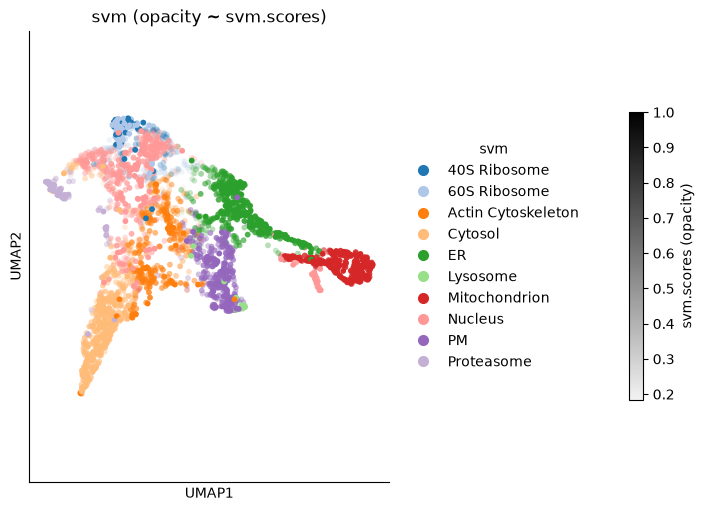
grassp’s plotting takes the column names as arguments, so pRoloc’s own names go straight in. The UMAP came back with the object, so there is nothing to recompute — here the SVM call with point transparency scaled by its confidence:

gr.pl.umap_prob(annotated, color="svm", color_prob="svm.scores", size=70)

<Axes: title={'center': 'svm (opacity ~ svm.scores)'}, xlabel='UMAP1', ylabel='UMAP2'>

Do the two frameworks agree?

grassp has its own RBF-SVM annotator, so we can give it the same data and the same markers and see how far apart the two land. Underneath, both wrap libsvm, so in principle this is the same estimator run twice.

Three things have to line up first, and none of them is about the bridge:

• Feature scaling, and therefore gamma. e1071 standardises every fraction by default (scale = TRUE); scikit-learn never does. Sum-normalised profiles sit around 0.1 with squared distances of ~1e-3, so pRoloc’s sigma = 0.1 — sensible on standardised data — leaves the kernel nearly constant on raw ones, and the two disagree on a third of all proteins. Scaling first is what makes the comparison meaningful, and then gr.tl.svm_train independently picks gamma = 0.1 too.

• Markers. pRoloc’s svm column has the markers pinned to their own labels, because MLearn only predicts the held-out proteins. fix_markers=True does the same here; without it we would be scoring grassp’s re-prediction of its own training set.

• Class weights. pRoloc passes none unless asked; grassp balances by default, so class_weight=None on both calls.

sc.pp.scale writes into .X, and the plots above want the profiles as they were — so park them in a layer, scale, and put them back afterwards.

annotated.layers["profiles"] = annotated.X.copy()  # keep the sum-normalised profiles
sc.pp.scale(annotated)  # z-score each fraction, as e1071 does internally

gr.tl.svm_train(
    annotated,
    gt_col="markers10",
    cv_splits=5,
    cv_repeats=20,
    class_weight=None,
    random_state=0,
)
print("grassp tuned on the scaled fractions:", annotated.uns["svm.params"]["best_params"])

gr.tl.svm_annotation(
    annotated,
    gt_col="markers10",
    fix_markers=True,  # as pRoloc does: markers keep their own label
    min_probability=0.0,  # no threshold, so every protein is called on both sides
    key_added="svm_grassp",
)

annotated.X = annotated.layers.pop("profiles")  # profiles back in place

same = annotated.obs["svm"].astype(str) == annotated.obs["svm_grassp"].astype(str)
predicted = annotated.obs["markers10"].isna()  # the rows pRoloc actually predicted
print(
    f"\nthe two agree on {same[predicted].mean():.1%} of the "
    f"{predicted.sum()} unlabelled proteins"
)

Fitting 100 folds for each of 54 candidates, totalling 5400 fits

grassp tuned on the scaled fractions: {'C': 8.0, 'gamma': 0.1}

the two agree on 92.4% of the 2147 unlabelled proteins

/Users/mfrank/code/grassp/.venv-dev/lib/python3.12/site-packages/sklearn/svm/_base.py:239: FutureWarning: The `probability` parameter was deprecated in 1.9 and will be removed in version 1.11. Use `CalibratedClassifierCV(SVC(), ensemble=False)` instead of `SVC(probability=True)`
  warnings.warn(

Around 92%, on two independently fitted models — grassp picked C = 8 where pRoloc was given 16 — and the last few percent are not a bridge problem either. libsvm is simply not a stable function of its inputs at this size: You can see this by repeatedly running the classifier in one of the frameworks. Even with the same matrix and same parameters, SVM reproduces top labels on 93.8% of these proteins.

annotated[annotated.obs["markers"].notna(), :].obs

	protein_name	gene_symbol	author_annotation	author_markers	bandle_probability	dl_candidate	author_markers_data10	marker_lilley	marker_christopher	marker_geladaki	...	harmonized_annotation_propagated	harmonized_annotation_propagated_probability	markers	markers10	svm	svm.scores	knn	knn.scores	svm_grassp	svm_grassp_probability
A0AVT1	Ubiquitin-like modifier-activating enzyme 6 (U...	UBA6	CYTOSOL	CYTOSOL	1.000000	NaN	CYTOSOL	Cytosol	Cytosol	Cytosol	...	Cytoplasm	1.000000	Cytosol	Cytosol	Cytosol	1.000000	Cytosol	1.0	Cytosol	1.000000
A6NDG6	Glycerol-3-phosphate phosphatase (G3PP) (EC 3....	PGP	CYTOSOL	NaN	0.695846	NaN	NaN	Cytosol	Cytosol	NaN	...	Cytoplasm	1.000000	Cytosol	Cytosol	Cytosol	1.000000	Cytosol	1.0	Cytosol	1.000000
O00116	Alkyldihydroxyacetonephosphate synthase, perox...	AGPS	PEROXISOME	PEROXISOME	1.000000	NaN	PEROXISOME	Peroxisome	Peroxisome	Peroxisome	...	Peroxisome	0.816999	Peroxisome	NaN	ER	0.817245	ER	1.0	ER	0.795697
O00161	Synaptosomal-associated protein 23 (SNAP-23) (...	SNAP23	PM	PM	1.000000	NaN	PM	PM	NaN	PM	...	Cell membrane	0.990546	PM	PM	PM	1.000000	PM	1.0	PM	1.000000
O00231	26S proteasome non-ATPase regulatory subunit 1...	PSMD11	PROTEASOME	PROTEASOME	1.000000	NaN	PROTEASOME	Proteasome	Proteasome	Proteasome	...	Proteasome	1.000000	Proteasome	Proteasome	Proteasome	1.000000	Proteasome	1.0	Proteasome	1.000000
...	...	...	...	...	...	...	...	...	...	...	...	...	...	...	...	...	...	...	...	...	...
Q9Y4P3	Transducin beta-like protein 2 (WS beta-transd...	TBL2	ER	ER	1.000000	NaN	ER	ER	ER	ER	...	Endoplasmic reticulum	0.963590	ER	ER	ER	1.000000	ER	1.0	ER	1.000000
Q9Y5B9	FACT complex subunit SPT16 (Chromatin-specific...	SUPT16H	CYTOSOL	NaN	0.999922	NaN	NaN	Nucleus	NaN	NaN	...	Nucleus	0.943463	Nucleus	Nucleus	Nucleus	1.000000	Nucleus	1.0	Nucleus	1.000000
Q9Y5L4	Mitochondrial import inner membrane translocas...	TIMM13	MITOCHONDRION	NaN	1.000000	NaN	NaN	Mitochondrion	Mitochondrion	Mitochondrion	...	Mitochondrion	0.985760	Mitochondrion	Mitochondrion	Mitochondrion	1.000000	Mitochondrion	1.0	Mitochondrion	1.000000
Q9Y617	Phosphoserine aminotransferase (EC 2.6.1.52) (...	PSAT1	CYTOSOL	CYTOSOL	1.000000	NaN	CYTOSOL	Cytosol	Cytosol	Cytosol	...	Cytoplasm	1.000000	Cytosol	Cytosol	Cytosol	1.000000	Cytosol	1.0	Cytosol	1.000000
Q9Y639	Neuroplastin (Stromal cell-derived receptor 1)...	NPTN	LYSOSOME	NaN	1.000000	DL candidate	NaN	PM	NaN	NaN	...	Cell membrane	0.933088	PM	PM	PM	1.000000	PM	1.0	PM	1.000000

403 rows × 32 columns

Reading pRolocdata without any R

Not every pRoloc dataset needs the bridge. pRolocdata is a Bioconductor package of curated MSnSets — the reference collection for pRoloc. They are distributed as R .rda files. grassp can also read those directly, with no R installation and no grasspio involved: gr.io.read_prolocdata parses R’s serialisation format with the pure-Python rdata package (pip install grassp[proloc]).

gr.ds.list_prolocdata_files() lists what is in the collection, straight from the repository:

prolocdata = gr.ds.list_prolocdata_files()

print(f"{len(prolocdata)} datasets available")
print("  Dunkley:", [name for name in prolocdata if "dunkley" in name.lower()])

144 datasets available
  Dunkley: ['dunkley2006', 'dunkley2006goCC']

gr.ds.download_prolocdata() fetches a dataset by name and hands back an AnnData. We’ll take dunkley2006, the Arabidopsis LOPIT experiment that gave the field its first published marker sets. It is not on the grassp portal, which starts at 2010 — so pRolocdata is how you reach the older literature.

dunkley = gr.ds.download_prolocdata("dunkley2006")
dunkley

AnnData object with n_obs × n_vars = 689 × 16
    obs: 'assigned', 'evidence', 'method', 'new', 'pd.2013', 'pd.markers', 'markers.orig', 'markers'
    var: 'membrane.prep', 'fraction', 'replicate'
    uns: 'dataset_name', 'file_name', 'MIAPE_metadata', 'processing', 'assigned_colors', 'pd.2013_colors', 'pd.markers_colors', 'markers.orig_colors', 'markers_colors'

The mapping is the same one as above, read backwards: fData became .obs, phenoData became .var, and the MSnSet’s experimentData is parked in .uns["MIAPE_metadata"]. Four marker columns came along — markers, markers.orig, pd.markers, pd.2013.

This path is also the one place grassp itself converts pRoloc’s "unknown" sentinel to NaN, since there is no R side to do it. It applies to every text column, so all four marker sets arrive usable by e.g. plotting functions:

# From here it is an ordinary AnnData, so scanpy applies. pRolocdata ships no embeddings, unlike
# the portal datasets, so compute one first.
sc.pp.pca(dunkley)
sc.pl.pca(dunkley, color=["markers", "markers.orig", "pd.markers", "pd.2013"], size=70)

Limitations

• .obsp/.varp are the only slots that cannot cross: eSet has no pairwise slot, and pRoloc’s one neighbour-ish representation (nndist()) writes flat positional indices, which are silently wrong after any subsetting. A graph is derived from .X, so gr.pp.neighbors rebuilds it if necessary.

• A class name containing / cannot be a DataFrame column, because HDF5 reads it as a path separator. So be careful with column names like: “Endoplasmic reticulum/Golgi apparatus”

• pRoloc does not always try to save all analysis results to the data object. For example, optimisation and MCMC side objects (GenRegRes, MAPParams, bandleParams) are returned, rather than added to the MSnSet. These reuslts do not get transferred back automatically.

• Nothing is renamed, so a column called svm in R is a column called svm here. If you want grassp’s own naming (svm_probabilities and friends), rename it yourself — the bridge deliberately does not guess.