
pRoloc integration: for pRoloc users#
The grassp data portal publishes over a hundred
curated subcellular fractionation datasets, uniformly processed, each with several published
marker sets already mapped onto it. They are stored as .h5ad, which sounds like a Python
format, but the grasspio R package (uses anndataR under the hood) can translate it to an MSnSet.
This means that you can use pRoloc to analyze and visualize a grassp dataset without ever leaving R.
So this tutorial needs no Python at all. You download a file, get an
MSnSet, and from there it is ordinary pRoloc. It also goes the other way: the last section
takes a pRolocdata object and writes it out as h5ad.
Note
This tutorial is for someone who works primarily in R and wants to use grassp’s data or a grassp method. If you work primarily in Python, read the companion tutorial instead: pRoloc integration: for grassp users.
Requirements#
install.packages(c("remotes", "BiocManager"))

# We need rdf5 to read the on disk h5ad format that grassp uses, and pRoloc/pRolocdata for the processing.
BiocManager::install(c("rhdf5", "pRoloc", "pRolocdata"))

# grasspio is a small R package that grassp provides to read/write h5ad files. It uses scVerse's anndataR package under the hood.
remotes::install_github("czbiohub-sf/grassp", subdir = "r/grasspio")
Note that grasspio requires R >=4.5.
suppressPackageStartupMessages({
  library(grasspio)
  library(pRoloc)
  library(MSnbase)
})
# IRkernel decides figure size from these rather than from knitr chunk options.
options(repr.plot.width = 9, repr.plot.height = 6, width = 100)
# Print results as an R console would, rather than as IRkernel's rich HTML.
options(jupyter.rich_display = FALSE)
Getting a dataset#
Browse the portal, pick a dataset, and take its
.h5ad. The files sit at a predictable URL, so you can download one in your browser or fetch it
from R:
https://public.czbiohub.org/proteinxlocation/datasets/<name>.h5ad       # processed
https://public.czbiohub.org/proteinxlocation/datasets_raw/<name>.h5ad   # pre-enrichment
The datasets/ objects are already preprocessed: enriched, replicates collapsed, and each
protein’s profile already normalised to sum to 1. The datasets_raw/ objects are raw intensities
with replicates preserved — useful, but they need normalising before pRoloc’s distance-based
methods mean anything.
Here we take Currie_2024_AC16_Control, a LOPIT-DC experiment on AC16 cardiomyocytes for demonstration.:
h5ad_path <- file.path(tempdir(), "Currie_2024_AC16_Control.h5ad")
download.file(
  "https://public.czbiohub.org/proteinxlocation/datasets/Currie_2024_AC16_Control.h5ad",
  h5ad_path,
  mode = "wb"
)
x <- grassp_as_msnset(h5ad_path, nan_to_unknown = TRUE)
x
MSnSet (storageMode: lockedEnvironment)
assayData: 2538 features, 10 samples
  element names: exprs, log_intensities, original_intensities, pvals
protocolData: none
phenoData
  sampleNames: F1 F2 ... F10 (10 total)
  varLabels: development_stage tissue ... PCs (33 total)
  varMetadata: labelDescription
featureData
  featureNames: A0AVT1 A1L0T0 ... Q9Y6Y8 (2538 total)
  fvarLabels: protein_name gene_symbol ... harmonized_annotation_propagated_probabilities
    (41 total)
  fvarMetadata: labelDescription
experimentData: use 'experimentData(object)'
Annotation:
- - - Processing information - - -
Imported from grassp h5ad [Currie_2024_AC16_Control.h5ad]: Fri Aug 14 11:27:29 2026
 MSnbase version: 2.36.0
That is the whole conversion. There is nothing special about the file: a portal dataset is a plain
h5ad (see the AnnData documentation for more info). The one thing grassp_as_msnset() does change is the
nan_to_unknown default, which rewrites NA markers to the literal "unknown" that pRoloc
assumes, because markerMSnSet() fails outright on NA.
Getting oriented#
Everything in the AnnData object has landed somewhere, slot for slot:
grassp |
pRoloc |
|---|---|
|
|
|
|
|
|
|
|
|
|
|
|
|
extra |
|
|
everything else in |
|
|
nothing — |
So per-protein annotations are fData, per-fraction ones are pData, and the extra matrices are
additional assayData elements:
dim(x)
head(fvarLabels(x), 12)
assayDataElementNames(x)
[1] 2538 10
 [1] "protein_name"          "gene_symbol"           "author_annotation"     "author_markers"
 [5] "bandle_probability"    "dl_candidate"          "author_markers_data10" "marker_lilley"
 [9] "marker_christopher"    "marker_geladaki"       "marker_itzhak"         "marker_villaneuva"
[1] "exprs" "log_intensities" "original_intensities" "pvals"
Some fData columns are themselves matrices — the per-protein × per-compartment arrays that
came from AnnData’s obsm. That is pRoloc’s own idiom for score matrices, so they arrive in the
shape pRoloc expects. Note that grassp stores PCA and UMAP coordinates in fData(x)$X_pca. This
means that plotting can be done cheaply without computing the dimensionality reduction again.
vapply(
  fData(x),
  function(col) if (is.matrix(col)) paste(dim(col), collapse = " x ") else "",
  character(1)
)[c("X_pca", "X_umap", "harmonized_annotation_propagated_probabilities")]
                                         X_pca                                         X_umap
                                    "2538 x 9"                                     "2538 x 2"
harmonized_annotation_propagated_probabilities
                                   "2538 x 16"
The publication metadata came too. An MSnSet has no slot for arbitrary key-value metadata, so
grasspio parks whatever it cannot map on experimentData(x)@other$grassp_uns:
uns <- experimentData(x)@other$grassp_uns
unlist(uns[c("title", "publication_journal", "publication_doi")])
                                       title                          publication_journal
                  "Currie_2024_AC16_Control"                      "Nature Communications"
                             publication_doi
"https://doi.org/10.1038/s41467-024-46600-5"
Pick a marker column — there is no single one#
The portal maps several published marker sets onto every dataset. They are the marker lists from
the papers themselves, matched onto each dataset’s protein IDs by grassp’s
pp.add_markers(), many of them imported from pRoloc::pRolocmarkers()
We can check which marker columns are present, how many classes each has, and how many proteins are labelled in each:
marker_cols <- grep("^marker_|^author_markers", fvarLabels(x), value = TRUE)
data.frame(
  column = marker_cols,
  classes = vapply(marker_cols, function(f) length(getMarkerClasses(x, fcol = f)), integer(1)),
  labelled = vapply(marker_cols, function(f) sum(fData(x)[[f]] != "unknown"), integer(1)),
  row.names = NULL
)
  column                classes labelled
1 author_markers        12       334
2 author_markers_data10 12       334
3 marker_lilley         12       403
4 marker_christopher    12       948
5 marker_geladaki       10       349
6 marker_itzhak         12       725
7 marker_villaneuva     12       426
8 marker_hein2025       20      2266
9 marker_hein2025_gt    16       756
We will use marker_lilley, the set that grassp imports from pRoloc::pRolocmarkers():
FCOL <- "marker_lilley"
getMarkerClasses(x, fcol = FCOL)
dim(markerMSnSet(x, fcol = FCOL))
c(missing = sum(is.na(exprs(x))), rows_summing_to_1 = sum(abs(rowSums(exprs(x)) - 1) < 1e-6))
 [1] "40S Ribosome"       "60S Ribosome"       "Actin Cytoskeleton" "Cytosol"
 [5] "ER"                 "Golgi"              "Lysosome"           "Mitochondrion"
 [9] "Nucleus"            "Peroxisome"         "PM"                 "Proteasome"
[1] 403 10
          missing rows_summing_to_1
                0              2538
No preprocessing is needed on an enriched object: filterNA() and normalise() could be applied here if you load a raw object.
One trap before you plot. pRoloc defaults to fcol = "markers", and a portal object has no
such column — so a bare plot2D(x) errors with fcol %in% fvarLabels(object) is not TRUE.
Always name your column, or pass fcol = NULL.
Plotting#
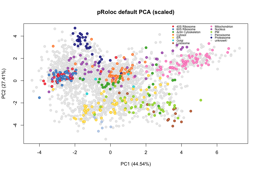
plot2D(x, fcol = FCOL, main = "pRoloc default PCA (scaled)")
addLegend(x, fcol = FCOL, where = "topright", cex = 0.6, ncol = 2)
options(repr.plot.height = 4)
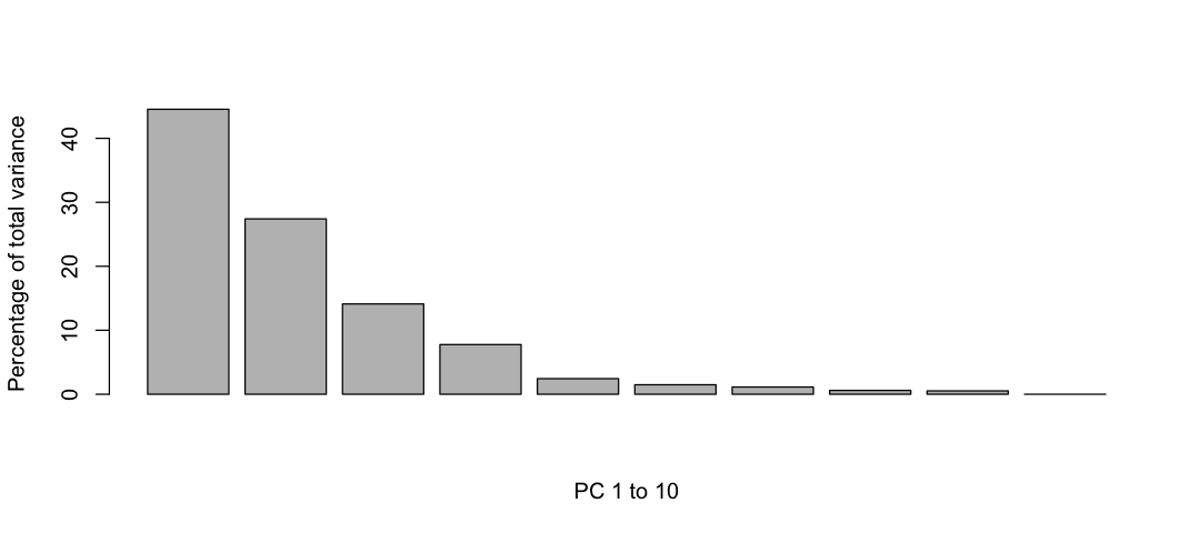
plot2D(x, method = "scree")
options(repr.plot.height = 6)
Comparing pRoloc’s PCA with the portal’s own#
The portal object already carries PCA coordinates in fData(x)$X_pca, computed by grassp when
the dataset was built. Recomputing them in pRoloc is a good way to check you are looking at the
same object — but only if you match the convention, and pRoloc’s default does not:
stored <- fData(x)$X_pca
colnames(stored) <- paste0("PC", seq_len(ncol(stored)))

default_pca <- plot2D(x, fcol = FCOL, plot = FALSE)
colnames(default_pca) # pRoloc prints the variance explained into the names
c(PC1 = cor(default_pca[, 1], stored[, 1]), PC2 = cor(default_pca[, 2], stored[, 2]))
[1] "PC1 (44.54%)" "PC2 (27.41%)"
      PC1       PC2
0.9198377 0.2361334
PC2 correlates at about 0.24. Nothing is broken: plot2D() passes scale = TRUE to prcomp,
scaling every fraction to unit variance, while the PCA in the grassp object was centered but not scaled. Scaling does not
merely stretch the axes — it changes the eigenvectors and their order, so comparing
component-by-component across the two conventions compares different directions.
Match the convention and they agree:
matched <- plot2D(x, fcol = FCOL, plot = FALSE, methargs = list(center = TRUE, scale = FALSE))
colnames(matched)
vapply(1:2, function(k) cor(matched[, k], stored[, k]), numeric(1))
[1] "PC1 (39.82%)" "PC2 (32.92%)"
[1] 1 -1
cor(PC2) = -1 is not a disagreement either. An eigenvector is only defined up to sign, so some
components come back negated; that is arithmetic, not a discrepancy. Fix it explicitly:
Drawing grassp’s embeddings with pRoloc#
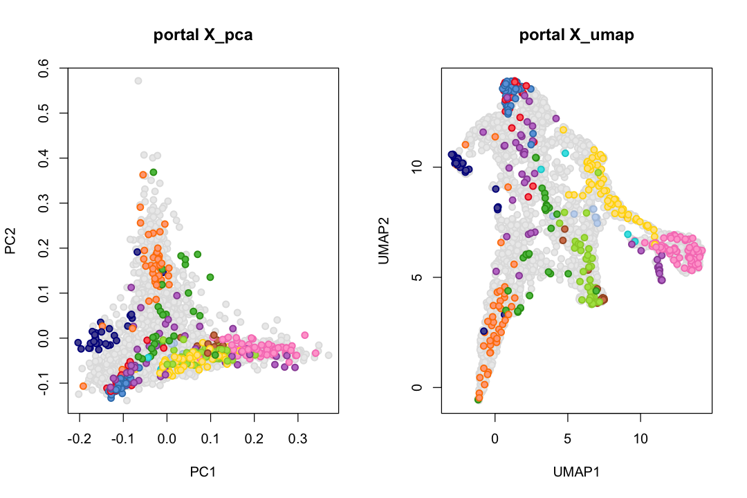
plot2D(method = "none") takes coordinates you already have and styles them like any other
pRoloc plot. That works for the stored PCA and, usefully, for the UMAP — which spares you
compiling a UMAP package just to look at it:
umap <- fData(x)$X_umap
colnames(umap) <- c("UMAP1", "UMAP2")
par(mfrow = c(1, 2))
plot2D(stored[, 1:2], method = "none", methargs = list(x), fcol = FCOL, main = "portal X_pca")
plot2D(umap, method = "none", methargs = list(x), fcol = FCOL, main = "portal X_umap")
par(mfrow = c(1, 1))
Profiles and marker quality#
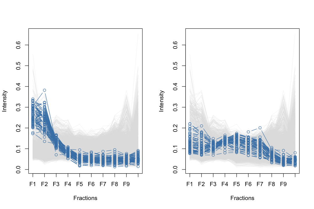
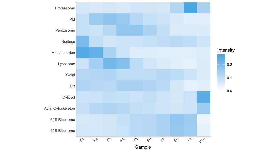
plotDist() draws one line per protein across the fractions, and markers = picks out a subset
to colour over the rest in grey. Passing the whole object and one compartment’s markers therefore
shows that compartment’s profile against the backdrop of everything measured — how distinctive
the profile is, and how tightly the markers agree with each other:
par(mfrow = c(1, 2))
for (cl in c("Mitochondrion", "ER")) {
  markers <- featureNames(x)[fData(x)[[FCOL]] == cl]
  plotDist(x, markers = markers, pch = 1,
           main = sprintf("%s (%d markers)", cl, length(markers)))
}
par(mfrow = c(1, 1))
options(repr.plot.height = 5)
plotConsProfiles(mrkConsProfiles(x, fcol = FCOL))
options(repr.plot.height = 6)
QSep() quantifies how well separated the marker classes are — the single most useful sanity
check on a fractionation experiment, and something the portal makes unusually easy because you
can ask it of every marker set at once. Higher is better: it is the between-class distance in
units of within-class spread, so a value near 1 means a class is no further from its neighbours
than from itself.
summary(QSep(x, fcol = FCOL))
sapply(marker_cols, function(f) median(summary(QSep(x, fcol = f), verbose = FALSE)))
   Min. 1st Qu.  Median    Mean 3rd Qu.    Max.
 0.8742  1.5359  2.3911  2.5345  3.1159  7.2937
       author_markers author_markers_data10         marker_lilley    marker_christopher
             3.173759              3.173759              2.391133              2.894165
      marker_geladaki         marker_itzhak     marker_villaneuva       marker_hein2025
             3.066839              1.703440              2.609419              1.634307
   marker_hein2025_gt
             1.719568
Classification#
svmClassification() needs hyperparameters. A real analysis gets them from svmOptimisation(),
which is a grid search over repeated stratified cross-validation and takes minutes, so it is
shown here but not run:
params <- svmOptimisation(x, fcol = FCOL, times = 100,
                          class.weights = classWeights(x, fcol = FCOL))
plot(params)
getParams(params)
set.seed(1) # e1071's probability scaling consumes the RNG; without this, runs differ
x <- svmClassification(x, fcol = FCOL, sigma = 0.1, cost = 16, scores = "all")

# `scores = "all"` writes the per-class matrix but NOT the scalar score that orgQuants() and
# getPredictions() look for, so derive it.
fData(x)$svm.scores <- apply(fData(x)$svm.all.scores, 1, max)
dim(fData(x)$svm.all.scores)
[1] "marker_lilley"
[1] 2538 12
The output columns are named svm, svm.scores, svm.all.scores regardless of which fcol you
trained on. The bare [1] "marker_lilley" above the result is a stray print() inside
MLInterfaces, not something you did.
# `mcol` is the second fcol-like trap: orgQuants() and getPredictions() default it to "markers"
# too, and use it to decide which proteins were training data.
ts <- orgQuants(x, fcol = "svm", scol = "svm.scores", mcol = FCOL, t = 0.75, verbose = FALSE)
ts[is.na(ts)] <- Inf # a class with too few markers has no quantile
x <- getPredictions(x, fcol = "svm", scol = "svm.scores", mcol = FCOL, t = ts, verbose = FALSE)
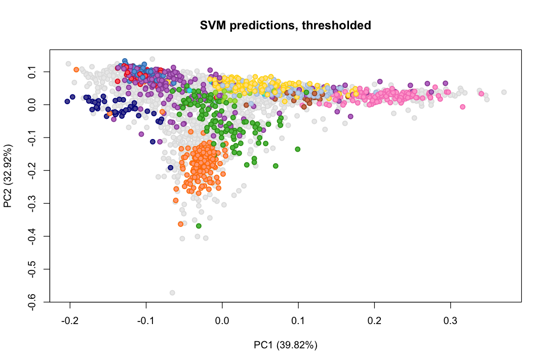
table(fData(x)$svm.pred == "unknown")
FALSE  TRUE
  941  1597
plot2D(x, fcol = "svm.pred", methargs = list(center = TRUE, scale = FALSE),
       main = "SVM predictions, thresholded")
A second classifier is a cheap sanity check, and QSep closes the loop quantitatively — do the
predicted labels separate better than the markers you started from?
set.seed(1)
x <- knnClassification(x, fcol = FCOL, k = 5) # note: knnClassification rejects `verbose`
c(svm_vs_knn_agreement = mean(fData(x)$svm == fData(x)$knn))
c(markers = median(summary(QSep(x, fcol = FCOL), verbose = FALSE)),
  svm.pred = median(summary(QSep(x, fcol = "svm.pred"), verbose = FALSE)))
[1] "marker_lilley"
svm_vs_knn_agreement
            0.822695
 markers svm.pred
2.391133 2.866938
Going the other way: a native pRoloc object out to h5ad#
The bridge is symmetric, and useful even if you never touch Python — neither pRoloc nor MSnbase
ships an h5ad exporter. Any MSnSet will do, including the ones pRolocdata distributes:
suppressPackageStartupMessages(library(pRolocdata))
data(dunkley2006)
dunkley2006
MSnSet (storageMode: lockedEnvironment)
assayData: 689 features, 16 samples
  element names: exprs
protocolData: none
phenoData
  sampleNames: M1F1A M1F4A ... M2F11B (16 total)
  varLabels: membrane.prep fraction replicate
  varMetadata: labelDescription
featureData
  featureNames: AT1G09210 AT1G21750 ... AT4G39080 (689 total)
  fvarLabels: assigned evidence ... markers (8 total)
  fvarMetadata: labelDescription
experimentData: use 'experimentData(object)'
  pubMedIds: 16618929
Annotation:
- - - Processing information - - -
Loaded on Thu Jul 16 22:53:08 2015.
Normalised to sum of intensities.
Added markers from  'mrk' marker vector. Thu Jul 16 22:53:08 2015
 MSnbase version: 1.17.12
out <- file.path(tempdir(), "dunkley2006.h5ad")
grassp_write_msnset(dunkley2006, out, overwrite = TRUE)
Wrote /var/folders/zk/39l3k6s15hz3z9k65hb14xpr0000gq/T//RtmpniKmjv/dunkley2006.h5ad (689 features x 16 fractions; 0 matrix column(s); 0 extra assay element(s)).
Back in Python:
  adata = anndata.read_h5ad("dunkley2006.h5ad")
Scalar fData columns become obs, matrix-valued ones become obsm data frames that carry their
own class names, extra assayData elements become layers, and "unknown" becomes NA on
the way out because that is grassp’s encoding. Reading it back gives the same object:
back <- grassp_as_msnset(out)
c(
  same_dim = identical(dim(back), dim(dunkley2006)),
  exprs_equal = isTRUE(all.equal(unname(exprs(back)), unname(exprs(dunkley2006)),
                                 tolerance = 1e-8)),
  same_columns = identical(sort(fvarLabels(back)), sort(fvarLabels(dunkley2006)))
)
getMarkerClasses(back, fcol = "markers")
    same_dim  exprs_equal same_columns
        TRUE         TRUE         TRUE
[1] "ER lumen"      "ER membrane"   "Golgi"         "Mitochondrion" "Plastid"       "PM"
[7] "Ribosome"      "TGN"           "vacuole"
That file is what a grassp user would open with anndata.read_h5ad("dunkley2006.h5ad") — no
grassp function required, because it is an ordinary h5ad. The mapping table, and the few things
that cannot cross, are in vignette("grasspio") and in IO: io.
Session info#
sessionInfo()
R version 4.5.3 (2026-03-11)
Platform: x86_64-apple-darwin13.4.0
Running under: macOS Tahoe 26.6

Matrix products: default
BLAS/LAPACK: /opt/homebrew/Caskroom/miniconda/base/envs/grassp-r64/lib/libopenblasp-r0.3.34.dylib;  LAPACK version 3.12.0

locale:
[1] C.UTF-8/C.UTF-8/C.UTF-8/C/C.UTF-8/C.UTF-8

time zone: America/Los_Angeles
tzcode source: system (macOS)

attached base packages:
[1] stats4    stats     graphics  grDevices utils     datasets  methods   base

other attached packages:
 [1] pRolocdata_1.48.0    pRoloc_1.51.1        BiocParallel_1.44.0  MLInterfaces_1.90.0
 [5] cluster_2.1.8.3      annotate_1.88.0      XML_3.99-0.23        AnnotationDbi_1.72.0
 [9] IRanges_2.44.0       MSnbase_2.36.0       ProtGenerics_1.42.0  S4Vectors_0.48.0
[13] mzR_2.44.0           Rcpp_1.1.1           Biobase_2.70.0       BiocGenerics_0.56.0
[17] generics_0.1.4       grasspio_0.1.0

loaded via a namespace (and not attached):
  [1] splines_4.5.3               pbdZMQ_0.3-14               filelock_1.0.3
  [4] tibble_3.3.1                hardhat_1.4.3               preprocessCore_1.72.0
  [7] pROC_1.19.0.1               rpart_4.1.27                lifecycle_1.0.5
 [10] httr2_1.3.0                 doParallel_1.0.17           globals_0.19.1
 [13] lattice_0.22-9              MASS_7.3-66                 MultiAssayExperiment_1.36.1
 [16] dendextend_1.19.1           magrittr_2.0.5              limma_3.66.0
 [19] plotly_4.12.1               otel_0.2.0                  reticulate_1.46.0
 [22] MsCoreUtils_1.22.1          DBI_1.3.0                   RColorBrewer_1.1-3
 [25] lubridate_1.9.5             abind_1.4-8                 GenomicRanges_1.62.1
 [28] purrr_1.2.2                 mixtools_2.0.0.1            AnnotationFilter_1.34.0
 [31] nnet_7.3-20                 ipred_0.9-15                lava_1.9.2
 [34] listenv_1.0.0               gdata_3.0.1                 parallelly_1.48.0
 [37] ncdf4_1.24                  codetools_0.2-20            DelayedArray_0.36.0
 [40] tidyselect_1.2.1            Spectra_1.20.1              farver_2.1.2
 [43] viridis_0.6.5               matrixStats_1.5.0           BiocFileCache_3.0.0
 [46] base64enc_0.1-6             Seqinfo_1.0.0               jsonlite_2.0.0
 [49] caret_7.0-1                 e1071_1.7-17                survival_3.8-9
 [52] iterators_1.0.14            foreach_1.5.2               segmented_2.2-1
 [55] tools_4.5.3                 progress_1.2.3              glue_1.8.1
 [58] prodlim_2026.03.11          gridExtra_2.3.1             SparseArray_1.10.8
 [61] BiocBaseUtils_1.12.0        xfun_0.60                   MatrixGenerics_1.22.0
 [64] IRdisplay_1.1               dplyr_1.2.1                 withr_3.0.3
 [67] BiocManager_1.30.27         fastmap_1.2.0               rhdf5filters_1.22.0
 [70] digest_0.6.39               timechange_0.4.0            R6_2.6.1
 [73] colorspace_2.1-3            gtools_3.9.5                lpSolve_5.6.23
 [76] biomaRt_2.66.1              RSQLite_3.53.3              tidyr_1.3.2
 [79] hexbin_1.28.6               data.table_1.18.4           recipes_1.3.3
 [82] FNN_1.1.4.1                 class_7.3-23                prettyunits_1.2.0
 [85] PSMatch_1.14.0              httr_1.4.8                  htmlwidgets_1.6.4
 [88] S4Arrays_1.10.1             ModelMetrics_1.2.2.2        pkgconfig_2.0.3
 [91] gtable_0.3.6                timeDate_4052.112           blob_1.3.0
 [94] S7_0.2.2                    impute_1.84.0               XVector_0.50.0
 [97] htmltools_0.5.9             MALDIquant_1.22.3           clue_0.3-68
[100] scales_1.4.0                png_0.1-9                   gower_1.0.2
[103] knitr_1.51                  MetaboCoreUtils_1.18.1      reshape2_1.4.5
[106] uuid_1.2-2                  coda_0.19-4.1               nlme_3.1-170
[109] curl_7.1.0                  anndataR_1.3.1              rhdf5_2.54.1
[112] repr_1.1.7                  proxy_0.4-29                cachem_1.1.0
[115] stringr_1.6.0               parallel_4.5.3              mzID_1.48.0
[118] vsn_3.78.1                  pillar_1.11.1               grid_4.5.3
[121] vctrs_0.7.3                 pcaMethods_2.2.0            randomForest_4.7-1.2
[124] dbplyr_2.6.0                xtable_1.8-8                evaluate_1.0.5
[127] mvtnorm_1.4-2               cli_3.6.6                   compiler_4.5.3
[130] rlang_1.3.0                 crayon_1.5.3                future.apply_1.20.2
[133] labeling_0.4.3              LaplacesDemon_16.1.8        mclust_6.1.3
[136] QFeatures_1.20.0            affy_1.88.0                 plyr_1.8.9
[139] fs_2.1.0                    stringi_1.8.9               viridisLite_0.4.3
[142] Biostrings_2.78.0           lazyeval_0.2.3              Matrix_1.7-5
[145] IRkernel_1.3.2              hms_1.1.4                   bit64_4.8.2
[148] future_1.75.0               Rhdf5lib_1.32.0             ggplot2_4.0.3
[151] KEGGREST_1.50.0             statmod_1.5.2               SummarizedExperiment_1.40.0
[154] kernlab_0.9-33              igraph_2.3.3                memoise_2.0.1
[157] affyio_1.80.0               sampling_2.11               bit_4.6.0