Ontology-aware annotation with “independent_diffusion”

grassp offers two graph-based annotation families, for two kinds of label:

	competitive_propagation	independent_diffusion
labels	mutually exclusive (one per protein)	overlapping / hierarchical (several per protein)
propagation	competitive (cross-normalized)	one-vs-rest, independent
output	a simplex (rows sum to 1)	per-term membership probabilities (no simplex)
resolution	argmax, built in	a separate step at the end
typical use	markers	GO-CC / UniProt-SL / COMPARTMENTS

This notebook demonstrates the elegant properties of independent_diffusion on simulated maps. Simulation is deliberate: we control how separated the compartments are and we know the ground truth exactly, so every claimed property can be shown as a clean curve.

We show five properties:

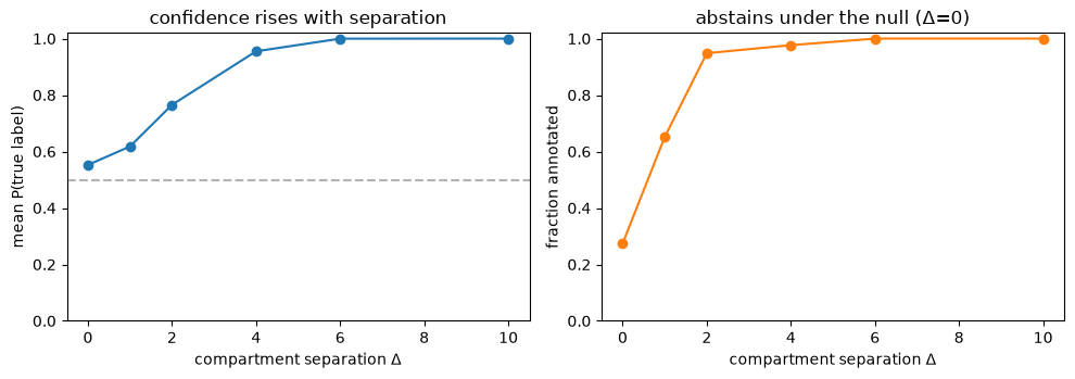
1. Confidence tracks data separation, and the method abstains under the null.

2. The confidence is honest (calibrated probabilities ≈ empirical membership).

3. Hierarchy resolves only when the data supports it (nucleus vs nucleolus).

4. Multi-localization: probabilities are non-simplex — a protein can be confidently in two places.

5. Calibrated confidence gives an FDR dial: thresholding trades coverage for precision.

Setup

import warnings

warnings.filterwarnings("ignore")
import numpy as np
import pandas as pd
import anndata as ad
import scanpy as sc
import matplotlib.pyplot as plt
import grassp as gr

sc.settings.verbosity = 0


def make_map(X, n_neighbors=15, seed=0, umap=False):
    """Wrap latent coordinates X (n_proteins x n_features) into an AnnData with a kNN
    graph in obsp['connectivities'] (what both annotation functions read), plus gene
    symbols and, optionally, a UMAP embedding for plotting."""
    genes = np.array([f"P{i}" for i in range(X.shape[0])])
    a = ad.AnnData(np.asarray(X, dtype=float))
    a.obs["gene_symbol"] = genes
    sc.pp.neighbors(a, n_neighbors=n_neighbors, random_state=seed)
    if umap:
        sc.tl.umap(a, random_state=seed)
    return a, genes

1. Confidence tracks data separation (and abstains under the null)

Two compartments whose centres we push apart by a separation Δ. At each Δ we diffuse the two gene sets one-vs-rest and read off (a) the mean calibrated probability of the true label and (b) the fraction of proteins that get any label at all. When Δ = 0 the two compartments are fully overlapping (the null): a protein’s neighbourhood is 50/50, so the probability sits at the base rate and the likelihood resolver abstains rather than guess.

seps = [0, 1, 2, 4, 6, 10]
d, npc = 15, 300
mean_true_P, coverage = [], []
for sep in seps:
    rng = np.random.RandomState(0)
    centers = np.zeros((2, d))
    centers[1, 0] = sep  # separation along one axis
    lab = np.repeat([0, 1], npc)
    X = centers[lab] + rng.randn(2 * npc, d)  # blob = centre + unit noise
    a, g = make_map(X)
    gene_sets = {"nucleus": list(g[lab == 0]), "mitochondrion": list(g[lab == 1])}
    gr.tl.independent_diffusion(a, gene_sets, gene_key="gene_symbol")
    P = a.obsm["ann_diffusion_probabilities"]
    cats = list(a.uns["ann_diffusion_categories"])
    true_col = [cats.index(["nucleus", "mitochondrion"][l]) for l in lab]
    mean_true_P.append(P[np.arange(len(lab)), true_col].mean())
    coverage.append(a.obs["ann_diffusion_resolved"].notna().mean())

fig, ax = plt.subplots(1, 2, figsize=(10, 3.6))
ax[0].plot(seps, mean_true_P, "o-")
ax[0].axhline(0.5, ls="--", c="0.7")
ax[0].set(
    xlabel="compartment separation Δ",
    ylabel="mean P(true label)",
    title="confidence rises with separation",
    ylim=(0, 1.02),
)
ax[1].plot(seps, coverage, "o-", color="C1")
ax[1].set(
    xlabel="compartment separation Δ",
    ylabel="fraction annotated",
    title="abstains under the null (Δ=0)",
    ylim=(0, 1.02),
)
plt.tight_layout()
plt.show()

# The same, as a map: colour = resolved label, opacity = confidence (maxp).
for sep, name in [(1, "barely separated"), (6, "well separated")]:
    rng = np.random.RandomState(0)
    centers = np.zeros((2, d))
    centers[1, 0] = sep
    lab = np.repeat([0, 1], npc)
    X = centers[lab] + rng.randn(2 * npc, d)
    a, g = make_map(X, umap=True)
    gene_sets = {"nucleus": list(g[lab == 0]), "mitochondrion": list(g[lab == 1])}
    gr.tl.independent_diffusion(a, gene_sets, gene_key="gene_symbol")
    gr.pp.set_sensible_compartment_colors(a, columns=["ann_diffusion_resolved"])
    axp = gr.pl.umap_prob(
        a,
        color="ann_diffusion_resolved",
        color_prob="ann_diffusion_maxp",
        prob_vmin=0.5,
        prob_vmax=1.0,
        show=False,
    )
    axp.set_title(f"Δ={sep} ({name})")
    plt.show()

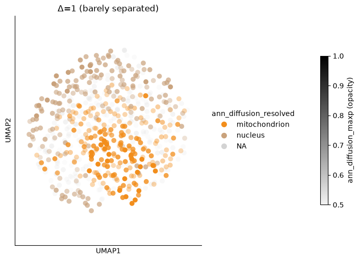
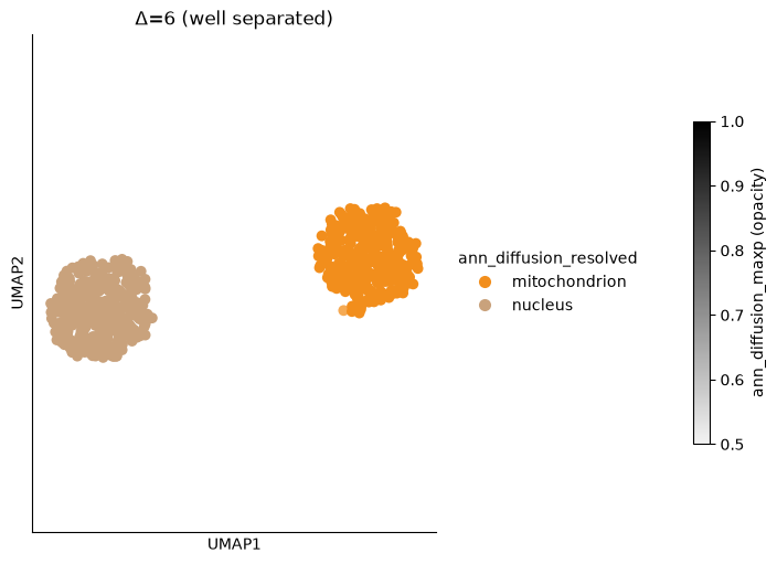
Takeaway. Confidence is not a fixed number — it grows as the compartments actually separate in the data, and collapses to abstention when there is no structure to read.

2. The confidence is honest (calibration)

Because we simulated the data we know each protein’s true membership, so we can check whether a reported probability means what it says. We diffuse four partially-overlapping compartments and compare the raw neighbourhood score (calibration="none") against the default "size_aware" calibration. A well-calibrated probability lies on the diagonal (of proteins called at probability p, a fraction p are truly members).

rng = np.random.RandomState(1)
d, npc, K = 20, 200, 4
centers = rng.randn(K, d) * 0.7  # partial overlap -> spread scores
lab = np.repeat(np.arange(K), npc)
X = centers[lab] + rng.randn(K * npc, d)
a, g = make_map(X)
gene_sets = {f"compartment {k}": list(g[lab == k]) for k in range(K)}
truth = np.stack([np.isin(g, gene_sets[t]) for t in gene_sets]).T.astype(float)


def reliability(P, Y, nbins=10, min_count=25):
    edges = np.linspace(0, 1, nbins + 1)
    idx = np.clip(np.digitize(P.ravel(), edges) - 1, 0, nbins - 1)
    Pr, Yr = P.ravel(), Y.ravel()
    xs, ys = [], []
    for b in range(nbins):
        s = idx == b
        if s.sum() >= min_count:
            xs.append(Pr[s].mean())
            ys.append(Yr[s].mean())
    return np.array(xs), np.array(ys)


def ece(P, Y, nbins=10):
    edges = np.linspace(0, 1, nbins + 1)
    idx = np.clip(np.digitize(P.ravel(), edges) - 1, 0, nbins - 1)
    Pr, Yr = P.ravel(), Y.ravel()
    tot = 0.0
    for b in range(nbins):
        s = idx == b
        if s.sum():
            tot += s.mean() * abs(Yr[s].mean() - Pr[s].mean())
    return tot


fig, ax = plt.subplots(figsize=(4.6, 4.6))
for cal, col in [("none", "C3"), ("size_aware", "C0")]:
    gr.tl.independent_diffusion(
        a, gene_sets, gene_key="gene_symbol", calibration=cal, resolve=None
    )
    P = a.obsm["ann_diffusion_probabilities"]
    xs, ys = reliability(P, truth)
    ax.plot(xs, ys, "o-", color=col, label=f"{cal}  (ECE={ece(P, truth):.3f})")
ax.plot([0, 1], [0, 1], "--", c="0.6")
ax.set(
    xlabel="predicted probability",
    ylabel="empirical membership",
    title="reliability",
    xlim=(0, 1),
    ylim=(0, 1),
)
ax.legend()
plt.tight_layout()
plt.show()

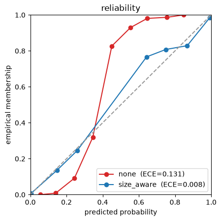
Takeaway. The raw neighbourhood fraction is informative but not calibrated (off the diagonal); size_aware maps it onto honest probabilities, so a stated confidence can be taken at face value.

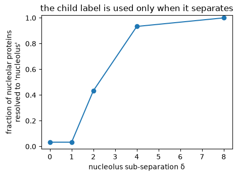
3. Hierarchy resolves only when the data supports it

A classic ontology problem: nucleolus is nested inside nucleus. We simulate a nuclear blob (plus a cytoplasmic background) and a nucleolar subset that we pull out of the nucleus by an increasing sub-separation δ. The gene sets are nested — nucleus contains the nucleolar proteins, nucleolus is the subset — and we resolve with the likelihood active-set resolver.

d = 20
n_cyto, n_nuc, n_olus = 300, 300, 120


def build_hier(delta, umap=False):
    """Cytoplasm background + nuclear bulk + a nucleolar subset shifted out by δ. Nested
    gene sets: 'nucleus' contains the nucleolar proteins; 'nucleolus' is the subset."""
    rng = np.random.RandomState(2)
    Xc = rng.randn(n_cyto, d)
    Xc[:, 1] += 12
    Xn = rng.randn(n_nuc, d)
    Xo = rng.randn(n_olus, d)
    Xo[:, 0] += delta
    X = np.vstack([Xc, Xn, Xo])
    a, g = make_map(X, umap=umap)
    gene_sets = {
        "cytoplasm": list(g[:n_cyto]),
        "nucleus": list(g[n_cyto:]),
        "nucleolus": list(g[n_cyto + n_nuc :]),
    }
    truth = np.array(["cytoplasm"] * n_cyto + ["nucleus"] * n_nuc + ["nucleolus"] * n_olus)
    return a, g, gene_sets, truth


deltas = [0, 1, 2, 4, 8]
frac_nucleolus = []
for delta in deltas:
    a, g, gene_sets, truth = build_hier(delta)
    gr.tl.independent_diffusion(a, gene_sets, gene_key="gene_symbol", resolve="likelihood")
    res = a.obs["ann_diffusion_resolved"].astype(object).values
    frac_nucleolus.append((res[truth == "nucleolus"] == "nucleolus").mean())

plt.figure(figsize=(4.8, 3.6))
plt.plot(deltas, frac_nucleolus, "o-")
plt.xlabel("nucleolus sub-separation δ")
plt.ylabel("fraction of nucleolar proteins\nresolved to 'nucleolus'")
plt.title("the child label is used only when it separates")
plt.ylim(-0.02, 1.02)
plt.tight_layout()
plt.show()

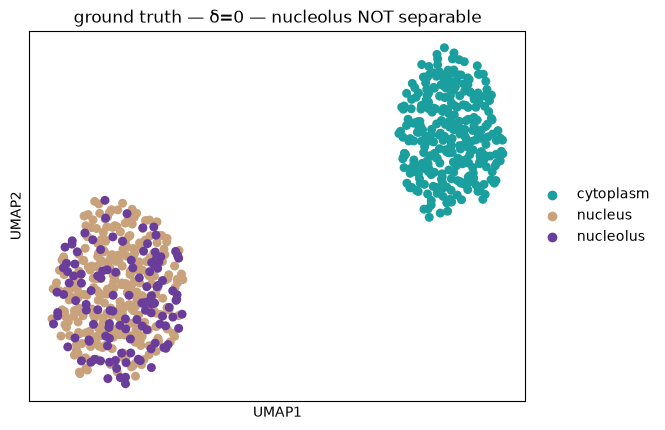
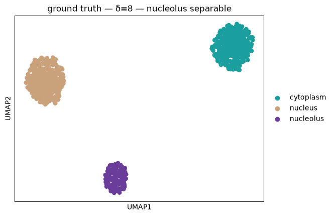
# Ground truth in BOTH regimes (colour = true fine label). At δ=0 the nucleolar proteins are
# intermixed with the nuclear bulk (no sub-structure to read); at δ=8 they form a distinct
# sub-cluster sitting inside the broader nuclear region (the labels are nested).
for delta, name in [(0, "δ=0 — nucleolus NOT separable"), (8, "δ=8 — nucleolus separable")]:
    a, g, gene_sets, truth = build_hier(delta, umap=True)
    a.obs["ground truth"] = pd.Categorical(
        truth, categories=["cytoplasm", "nucleus", "nucleolus"]
    )
    gr.pp.set_sensible_compartment_colors(a, columns=["ground truth"])
    sc.pl.umap(a, color="ground truth", title=f"ground truth — {name}")

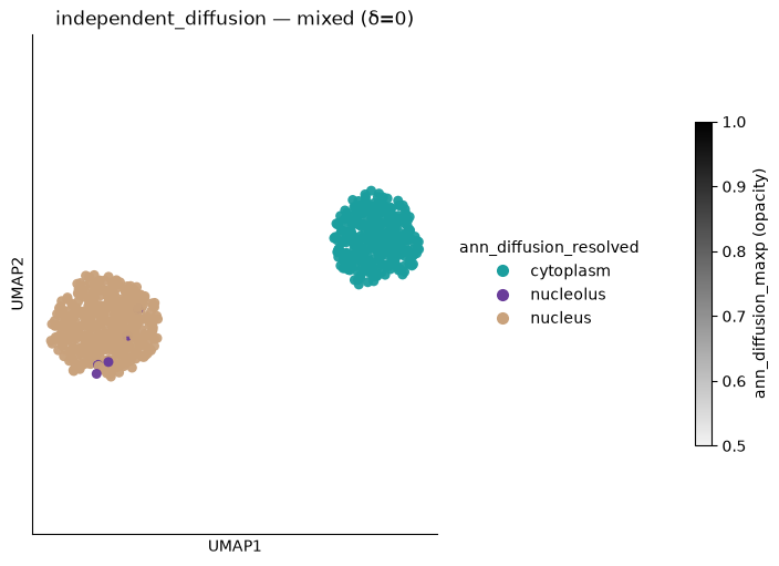
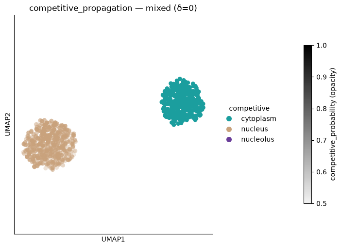
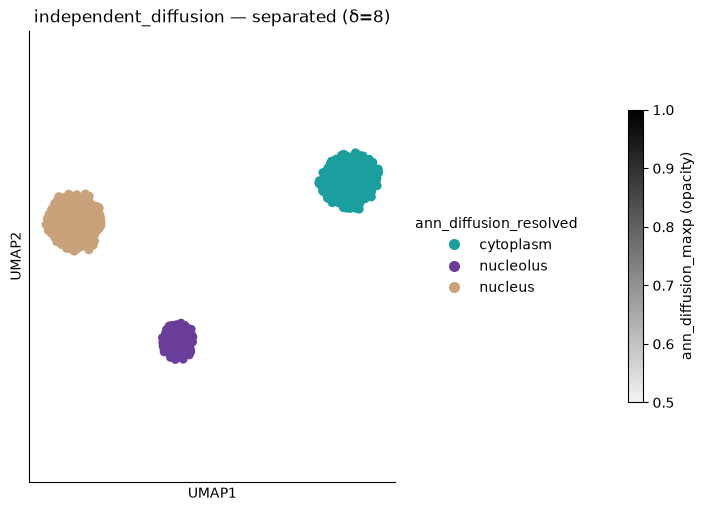
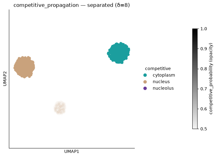
# Resolved maps for BOTH algorithms in BOTH regimes. Colour = resolved label, opacity =
# confidence. independent_diffusion resolves the nucleolus once it separates (δ=8);
# competitive_propagation leaves that region as low-confidence 'nucleus' — the 50/50 split
# loses to the parent at argmax, so the child label is never used.
cats3 = ["cytoplasm", "nucleus", "nucleolus"]
for delta, name in [(0, "mixed (δ=0)"), (8, "separated (δ=8)")]:
    a, g, gene_sets, truth = build_hier(delta, umap=True)
    gr.tl.independent_diffusion(a, gene_sets, gene_key="gene_symbol", resolve="likelihood")
    seed = np.zeros((a.n_obs, 3))
    seed[:n_cyto, 0] = 1
    seed[n_cyto:, 1] = 1
    seed[n_cyto + n_nuc :, 2] = 1  # nested seed
    a.obsm["nested_seed"] = seed
    a.uns["nested_seed_categories"] = cats3
    gr.tl.competitive_propagation(
        a,
        gt_col=None,
        seed_obsm_key="nested_seed",
        seed_categories_uns_key="nested_seed_categories",
        key_added="competitive",
        class_balance=False,
        min_probability=0,
        plot_optimization=False,
        verbose=False,
    )
    gr.pp.set_sensible_compartment_colors(a, columns=["ann_diffusion_resolved", "competitive"])
    ax1 = gr.pl.umap_prob(
        a,
        color="ann_diffusion_resolved",
        color_prob="ann_diffusion_maxp",
        prob_vmin=0.5,
        prob_vmax=1.0,
        show=False,
    )
    ax1.set_title(f"independent_diffusion — {name}")
    plt.show()
    ax2 = gr.pl.umap_prob(
        a,
        color="competitive",
        color_prob="competitive_probability",
        prob_vmin=0.5,
        prob_vmax=1.0,
        show=False,
    )
    ax2.set_title(f"competitive_propagation — {name}")
    plt.show()

Quantifying the 50/50 split

The maps make it visual; the bars below quantify it. For the nucleolar proteins we compare each algorithm’s P(nucleus) and P(nucleolus) — when the nucleolus is not separable (δ=0) and when it is (δ=8). Forced onto a simplex, competitive_propagation cannot express “in the nucleolus and therefore in the nucleus”, so its probability splits between the two.

cats3 = ["cytoplasm", "nucleus", "nucleolus"]
fig, axes = plt.subplots(1, 2, figsize=(9.5, 3.8), sharey=True)
for ax, (delta, name) in zip(axes, [(0, "δ=0 — not separable"), (8, "δ=8 — separable")]):
    a, g, gene_sets, truth = build_hier(delta)
    olus = truth == "nucleolus"
    gr.tl.independent_diffusion(a, gene_sets, gene_key="gene_symbol", resolve="likelihood")
    Pi = a.obsm["ann_diffusion_probabilities"]
    ci = list(a.uns["ann_diffusion_categories"])
    seed = np.zeros((a.n_obs, 3))
    seed[:n_cyto, 0] = 1
    seed[n_cyto:, 1] = 1
    seed[n_cyto + n_nuc :, 2] = 1  # nested seed
    a.obsm["nested_seed"] = seed
    a.uns["nested_seed_categories"] = cats3
    gr.tl.competitive_propagation(
        a,
        gt_col=None,
        seed_obsm_key="nested_seed",
        seed_categories_uns_key="nested_seed_categories",
        key_added="competitive",
        class_balance=False,
        min_probability=0,
        plot_optimization=False,
        verbose=False,
    )
    Pc = a.obsm["competitive_probabilities"]
    ind = [Pi[olus, ci.index("nucleus")].mean(), Pi[olus, ci.index("nucleolus")].mean()]
    comp = [Pc[olus, 1].mean(), Pc[olus, 2].mean()]  # cols: cyto, nuc, olus
    x = np.arange(2)
    w = 0.35
    ax.bar(x - w / 2, ind, w, label="independent_diffusion")
    ax.bar(x + w / 2, comp, w, color="C3", label="competitive_propagation")
    ax.axhline(0.5, ls="--", c="0.7")
    ax.set_xticks(x)
    ax.set_xticklabels(["P(nucleus)", "P(nucleolus)"])
    ax.set_title(name)
    ax.set_ylim(0, 1.05)
axes[0].set_ylabel("mean probability\n(nucleolar proteins)")
axes[0].legend(fontsize=8)
fig.suptitle(
    "resolving nucleus vs nucleolus — independent commits when the data allows; "
    "competitive is stuck on the simplex"
)
plt.tight_layout()
plt.show()

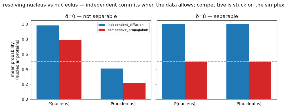
Takeaway. When the nucleolus is not separable (δ=0) both methods stay on nucleus: independent_diffusion reports P(nucleolus) ≈ 0.4 — honestly below the 0.5 call threshold — and falls back to the parent. When it is separable (δ=8) independent_diffusion drives both memberships to ≈1 and the likelihood resolver explains away the parent to commit to nucleolus, whereas competitive_propagation, bound to the simplex, is stuck at a 50/50 split and cannot use the child label even though the data clearly supports it. The child is used exactly when — and only when — the data supports it; the simplex constraint is what stops the competitive algorithm from ever getting there.

4. Multi-localization: non-simplex probabilities

Independent one-vs-rest diffusion does not force labels to compete, so a genuinely dual-localized protein can be confidently assigned to both compartments. Here a set of proteins sits between two compartments and is a member of both gene sets. We contrast independent_diffusion with competitive_propagation, which is constrained to a simplex.

rng = np.random.RandomState(3)
d, npc, ndual = 20, 250, 120
cA = np.zeros(d)
cB = np.zeros(d)
cB[0] = 12
X = np.vstack(
    [cA + rng.randn(npc, d), cB + rng.randn(npc, d), (cA + cB) / 2 + rng.randn(ndual, d) * 0.8]
)  # dual set at the midpoint
a, g = make_map(X)
dual = np.zeros(X.shape[0], bool)
dual[2 * npc :] = True
gene_sets = {
    "ER": list(g[:npc]) + list(g[dual]),
    "mitochondrion": list(g[npc : 2 * npc]) + list(g[dual]),
}

gr.tl.independent_diffusion(a, gene_sets, gene_key="gene_symbol", resolve=None)
Pind = a.obsm["ann_diffusion_probabilities"]
ci = list(a.uns["ann_diffusion_categories"])
iA, iB = ci.index("ER"), ci.index("mitochondrion")

a.obs["primary"] = np.array(
    ["ER"] * npc + ["mitochondrion"] * npc + [None] * ndual, dtype=object
)
gr.tl.competitive_propagation(
    a, gt_col="primary", plot_optimization=False, verbose=False, min_probability=0
)
Pc = a.obsm["competitive_propagation_probabilities"]
cc = list(a.obs["primary"].astype("category").cat.categories)
jA, jB = cc.index("ER"), cc.index("mitochondrion")

fig, ax = plt.subplots(1, 2, figsize=(9, 4.3), sharex=True, sharey=True)
ax[0].scatter(Pind[dual, iA], Pind[dual, iB], s=12, alpha=0.5)
ax[0].set(
    title=f"independent_diffusion\ndual-protein P(A)+P(B) ≈ {Pind[dual][:, [iA, iB]].sum(1).mean():.2f}",
    xlabel="P(ER)",
    ylabel="P(mitochondrion)",
)
ax[1].scatter(Pc[dual, jA], Pc[dual, jB], s=12, alpha=0.5, color="C3")
ax[1].set(
    title=f"competitive_propagation\nforced simplex, sum ≈ {Pc[dual][:, [jA, jB]].sum(1).mean():.2f}",
    xlabel="P(ER)",
)
for x in ax:
    x.plot([0, 1], [1, 0], "--", c="0.7")
    x.set_xlim(-0.02, 1.02)
    x.set_ylim(-0.02, 1.02)
plt.tight_layout()
plt.show()

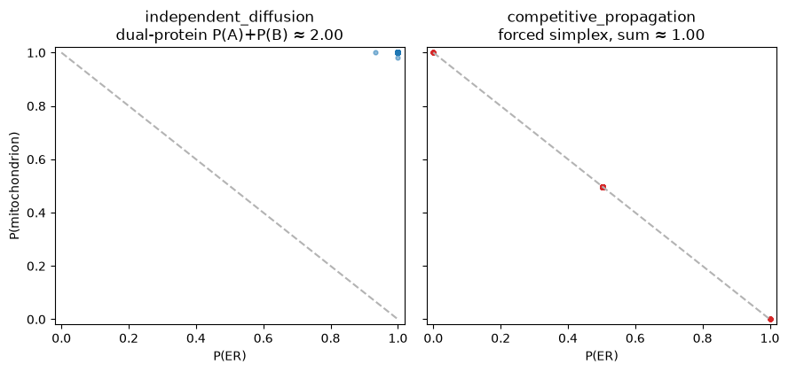
Takeaway. The dual proteins land in the top-right under independent_diffusion (high P for both ER and mitochondrion), but on the anti-diagonal under competitive_propagation, which must split one unit of probability. Overlapping biology needs non-simplex probabilities.

5. Calibrated confidence gives an FDR dial

Because the probability is calibrated, thresholding it at a confidence θ controls the false-positive rate: calls kept at P ≥ θ have empirical precision ≥ θ. Raising θ trades coverage for precision — the biologist picks the operating point.

rng = np.random.RandomState(4)
d, npc, K = 20, 200, 4
centers = rng.randn(K, d) * 0.4  # heavy overlap -> real FP to control
lab = np.repeat(np.arange(K), npc)
X = centers[lab] + rng.randn(K * npc, d)
a, g = make_map(X)
gene_sets = {f"compartment {k}": list(g[lab == k]) for k in range(K)}
truth = np.stack([np.isin(g, gene_sets[t]) for t in gene_sets]).T.astype(bool)
gr.tl.independent_diffusion(a, gene_sets, gene_key="gene_symbol", resolve=None)
P = a.obsm["ann_diffusion_probabilities"]

thetas = np.linspace(0.3, 0.95, 14)
prec_cum, prec_bin, coverage = [], [], []
for th in thetas:
    keep = P >= th  # cumulative: everything above θ
    prec_cum.append((keep & truth).sum() / max(keep.sum(), 1))
    coverage.append(keep.any(1).mean())
    near = (P >= th) & (P < th + 0.1)  # per-bin: calls with P ≈ θ
    prec_bin.append((near & truth).sum() / near.sum() if near.sum() >= 15 else np.nan)

fig, ax = plt.subplots(figsize=(5.4, 3.9))
ax.plot(
    thetas, prec_bin, "^-", color="C2", label="precision of calls with P ≈ θ  (calibration)"
)
ax.plot(thetas, prec_cum, "o-", label="precision of calls kept at P ≥ θ")
ax.plot(thetas, coverage, "s-", color="C1", label="coverage")
ax.plot([0.3, 1.0], [0.3, 1.0], "--", c="0.7", label="perfect calibration (precision = θ)")
ax.set(
    xlabel="confidence threshold θ  (= 1 − FDR)",
    ylabel="rate",
    title="calibrated probability as an FDR dial",
)
ax.legend(fontsize=8)
plt.tight_layout()
plt.show()

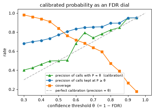
Takeaway. The per-bin precision (calls with P ≈ θ) lies on the diagonal — the probability means exactly what it says. The cumulative precision (everything kept at P ≥ θ) sits above the diagonal, because that set pools all calls with P in [θ, 1] whose average probability is

θ; that is not conservatism from miscalibration but the one-sided guarantee you want — thresholding at P ≥ 1 − FDR keeps calls at a realized FDR ≤ the target, and coverage falls as you tighten θ.

Summary

property	what it shows
§1 confidence vs separation	confidence reflects real neighbourhood structure; abstains under the null
§2 calibration	reported probabilities are honest (≈ empirical membership)
§3 hierarchy	nested labels resolve to the child only when it separates in the data
§4 multi-localization	non-simplex probabilities represent genuine dual localization
§5 FDR dial	thresholding calibrated P controls the false-positive rate

Which to use? Reach for competitive_propagation when labels are mutually exclusive and single-per-protein (e.g. curated markers); reach for independent_diffusion when labels overlap or are hierarchical (GO-CC, UniProt-SL, COMPARTMENTS).

On real maps, pass a real vocabulary — a {term: [genes]} dict, a .gmt path, or an Enrichr library name — e.g. gr.tl.independent_diffusion(adata, "path/to/GO_CC.gmt"), after loading a dataset with gr.ds.load_dataset(...). Note that the default size_aware calibration is designed for the messiness of real gene sets (incomplete membership, small terms, cross-fit noise); on the idealized simulations above its extra machinery is unnecessary, but on real ontologies it is what keeps small, sparsely-annotated terms from becoming over-confident.